Signal Classification by Sweeping Hyperparameters
This example shows how to use a preconfigured template in the Experiment Manager app to set up a signal classification experiment involving time-frequency features. The goal of the experiment is to train a classifier to determine if an electrocardiogram (ECG) signal exhibits arrhythmia, congestive heart failure, or normal sinus rhythm. The training and testing data consists of 96 ECG recordings from the MIT-BIH Arrhythmia Database, 30 recordings from the BIDMC Congestive Heart Failure Database, and 36 recordings from the MIT-BIH Normal Sinus Rhythm Database [1], [2], [3].
Experiment Manager (Deep Learning Toolbox) enables you to train networks with different hyperparameter combinations and compare results as you search for the specifications that best solve your problem. Signal Processing Toolbox™ provides preconfigured templates that you can use to quickly set up signal processing experiments. For more information about Experiment Manager templates, see Quickly Set Up Experiment Using Preconfigured Template (Deep Learning Toolbox).
Open Experiment
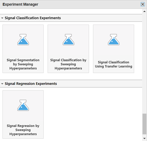
First, open the template. In the Experiment Manager toolstrip, click
New and select Project. In the dialog box,
click Blank Project, scroll to the Signal Classification
Experiments section, click Signal Classification by Sweeping
Hyperparameters, and optionally specify a name for the project folder.
Built-in training experiments consist of a description, an initialization function, a table of hyperparameters, a setup function, a collection of metric functions to evaluate the results of the experiment, and a set of supporting files.
The Description field contains a textual description of the experiment. For this example, the description is:
Signal Classification by Sweeping Hyperparameters
The Hyperparameters section specifies the strategy and
hyperparameter values to use. This experiment follows the Exhaustive
Sweep strategy, in which Experiment Manager trains the network
using every combination of hyperparameter values specified in the hyperparameter table. In
this case, the experiment has two hyperparameters:
featureTypespecifies the feature to extract from each signal and use to train the network. The options are:"stft"— Extract the short-time Fourier transform of each signal and use the transforms to train the network."cwt"— Extract the continuous wavelet transform of each signal and use the transforms to train the network.
initialLearnRatespecifies the initial learning rate. If the learning rate is too low, then training can take a long time. If the learning rate is too high, then training might reach a suboptimal result or diverge. The options are1e-3and1e-2.
The Setup Function section specifies a function that
configures the training data, network architecture, and training options for the experiment.
To open the Setup Function in the MATLAB® Editor, click Edit. The input to the setup function is
params, a structure with fields from the hyperparameter table. The
function returns four outputs that the experiment passes to trainnet (Deep Learning Toolbox):
dsTrain— A datastore that contains the training signals and their corresponding labelslayers— A layer array that defines the neural network architecturelossFcn— A cross-entropy loss function for classification tasks, returned as"crossentropy"options— AtrainingOptionsobject that contains training algorithm details
In this example, the setup function has these sections:
Download and Load Training Data downloads the data files into the temporary directory for the system and creates a signal datastore that points to the data set.
Resize Data resizes the data to a specific input size, if required by your model or feature extraction methods.
Extract Features uses
params.featureTypeto specify the feature extraction function. The continuous wavelet transform (CWT) and the Fourier synchrosqueezed transform (FSST) both have the same time resolution as the input signals.Split Data splits the data into training and validation sets.
Read Data into Memory loads all your data into memory to speed up the training process, if your system has enough resources.
Define Network Architecture creates a neural network using an array of layers that includes a bidirectional long short-term memory (BiLSTM) layer and a fully connected layer. For more information, see Example Deep Learning Network Architectures (Deep Learning Toolbox).
Define Training Hyperparameters calls
trainingOptions(Deep Learning Toolbox) to set the hyperparameters to use when training the network.Supporting Functions includes functionality for feature extraction and data resizing.
The Post-Training Custom Metrics section specifies optional functions that Experiment Manager evaluates each time it finishes training the network. This experiment does not include metric functions.
The Supporting Files section enables you to identify, add, or remove files required by your experiment. This experiment does not use supporting files.
Run Experiment
When you run the experiment, Experiment Manager repeatedly trains the network defined by the setup function. Each trial uses a different combination of hyperparameter values. By default, Experiment Manager runs one trial at a time. If you have Parallel Computing Toolbox™, you can run multiple trials at the same time or offload your experiment as a batch job in a cluster.
To run one trial of the experiment at a time, on the Experiment Manager toolstrip, set Mode to
Sequentialand click Run.To run multiple trials at the same time, set Mode to
Simultaneousand click Run. For more information, see Run Experiments in Parallel (Deep Learning Toolbox).To offload the experiment as a batch job, set Mode to
Batch SequentialorBatch Simultaneous, specify your cluster and pool size, and click Run. For more information, see Offload Experiments as Batch Jobs to a Cluster (Deep Learning Toolbox).
A table of results displays the training accuracy, training loss, validation accuracy, and validation loss values for each trial.
Evaluate Results
To find the best result for your experiment, sort the table of results by validation accuracy:
Point to the Validation Accuracy column.
Click the triangle ▼ icon.
Select Sort in Descending Order.
The trial with the highest validation accuracy appears at the top of the results table.
To record observations about the results of your experiment, add an annotation:
In the results table, right-click the Validation Accuracy cell of the best trial.
Select
Add Annotation.In the Annotations pane, enter your observations in the text box.
For each experiment trial, Experiment Manager produces a training progress plot, a confusion matrix for training data, and a confusion matrix for validation data. To see one of those plots, select the trial and click the corresponding button in the Review Results gallery on the Experiment Manager toolstrip.
Close Experiment
In the Experiment Browser pane, right-click the experiment name and select Close Project. Experiment Manager closes the experiment and the results contained in the project.
Setup Function
Download and Load Training Data
If you intend to place the data files in a folder different from the temporary
directory, replace tempdir with your folder name. To limit the run
time, this experiment uses only 40% of the data. To use more data, increase the value of
dataRatio.
function [dsTrain,layers,lossFcn,options] = Experiment_setup(params)

dataURL = "https://raw.githubusercontent.com/mathworks/physionet_ECG_data/main/ECGData.zip";
datasetFolder = fullfile(tempdir,"PhysionetECGData");
if ~exist(datasetFolder,"dir")
     mkdir(datasetFolder)
     zipFile = websave(tempdir,dataURL);
     unzip(zipFile,datasetFolder)
     delete(zipFile)
end

ECGData = importdata(fullfile(datasetFolder,"ECGData.mat"));
data = ECGData.Data;
numSignals = size(data,1);
data = mat2cell(data,ones(numSignals,1),size(data,2));
labels = ECGData.Labels;
labels = categorical(labels);
ds = combine(signalDatastore(data,SampleRate=128),arrayDatastore(labels));

rng("default")
dataRatio = 0.4;
idx = splitlabels(labels,dataRatio);
ds = subset(ds,idx{1});
labels = labels(idx{1});
Resize Data
If your model or feature extraction methods require no specific signal length, comment out this line.
ds= transform(ds,@helperResizeData);
Extract Features
In classification tasks, it is generally better to use extracted time-frequency features rather than raw signals because they highlight important information in the data and are thus better suited to identify and learn patterns. This experiment tries both the short-time Fourier transform and the continuous wavelet transform as extracted time-frequency features.
dsFeature = transform(ds,@(x)helperExtractFeatures(x,FeatureType=params.featureType));
feature = preview(dsFeature);
featureSize = size(feature{1});
Split Data
The experiment uses the training set to train the model. Use 80% of the data for the training set.
The experiment uses the validation set to evaluate the performance of the trained model during hyperparameter tuning. Use the remaining 20% of the data for the validation set.
If you intend to evaluate the generalization performance of your finalized model, set aside some data for testing as well.
trainValIdx = splitlabels(labels,[0.8,0.2]);
trainIdx = trainValIdx{1};
validIdx = trainValIdx{2};
dsTrain = subset(dsFeature,trainIdx);
dsValid = subset(dsFeature,validIdx);
Read Data into Memory
If the data does not fit into memory, set fitMemory to
false.
fitMemory = true;
if fitMemory
    dataTrain = readall(dsTrain);
    XTrain = signalDatastore(dataTrain(:,1));
    TTrain = arrayDatastore(vertcat(dataTrain(:,2)),OutputType="same");
    dsTrain = combine(XTrain,TTrain);

    dataValid = readall(dsValid);
    XValid = signalDatastore(dataValid(:,1));
    TValid = arrayDatastore(vertcat(dataValid(:,2)),OutputType="same");
    dsValid = combine(XValid,TValid);
end
Define Network Architecture
Create a small neural network using an array of layers. For classification tasks, use cross-entropy loss.
numF = 4;
numClasses = length(unique(labels));
layers = [
    imageInputLayer(featureSize,Normalization="none")

    convolution2dLayer(5,numF,Padding="same")
    batchNormalizationLayer
    reluLayer
    maxPooling2dLayer(3,Stride=2,Padding="same")

    convolution2dLayer(3,2*numF,Padding="same")
    batchNormalizationLayer
    reluLayer
    maxPooling2dLayer(3,Stride=2,Padding="same")

    convolution2dLayer(3,4*numF,Padding="same")
    batchNormalizationLayer
    reluLayer

    convolution2dLayer(3,4*numF,Padding="same")
    batchNormalizationLayer
    reluLayer

    averagePooling2dLayer(2)

    dropoutLayer(0.3)
    fullyConnectedLayer(numClasses)
    softmaxLayer
    ];

lossFcn = "crossentropy";
Define Training Hyperparameters
To set the batch size of the data for training, set
MiniBatchSizeto 20.To use the adaptive moment estimation (Adam) optimizer, specify the
"adam"option.To specify the initial learning rate, use
params.initialLearnRate.To use the parallel pool to read the transformed datastore, set
PreprocessingEnvironmentto"parallel".
miniBatchSize = 20;
options = trainingOptions("adam", ...
    InitialLearnRate=params.initialLearnRate, ...
    MaxEpochs=80, ...
    LearnRateSchedule="piecewise", ...
    LearnRateDropFactor=0.9, ...
    LearnRateDropPeriod=10, ...
    MiniBatchSize=miniBatchSize, ...
    Shuffle="every-epoch", ...
    Plots="training-progress", ...
    Metrics="accuracy", ...
    Verbose=false, ...
    ValidationData=dsValid, ...
    ExecutionEnvironment="auto", ...
    PreprocessingEnvironment="serial");
end
Supporting Functions
helperExtractFeatures function. Extract the features to use for training the network.
inputCellis a two-element cell array that contains an ECG signal vector and a categorical label.outputCellis a two-element cell array that contains the ECG signal features and a categorical label.
Compute time-frequency maps by using stft or
cwt (Wavelet Toolbox). In the cwt case,
resize the
feature.
function outputCell = helperExtractFeatures(inputCell,Nvargs)
    arguments
        inputCell
        Nvargs.FeatureType = "stft"
    end
    Fs = 128;
    sigs = inputCell(:,1);
    features = cell(size(sigs));
    switch Nvargs.FeatureType
        case "stft"
            for idx = 1:length(sigs)
                [s,f] = stft(sigs{idx},Fs,"FrequencyRange","onesided");
                findices = (f > 0.5) & (f < 40);
                features{idx} = abs(s(findices,:));
            end
        case "cwt"
            for idx = 1:length(sigs)
                [s,f] = cwt(sigs{idx},Fs);
                findices = (f > 0.5) & (f < 40);
                features{idx} = imresize(abs(s(findices,:)),[64,1024]);
            end
    end
    outputCell = [features inputCell(:,2)];
end
helperResizeData function. Pad or truncate an input ECG signal into targetLength-sample segments.
inputCellis a two-element cell array that contains an ECG signal and a label.outputCellis a two-column cell array that contains same-length labeled signal segments.
Pad or truncate the data to the target length and normalize it.
function outputCell = helperResizeData(inputCell)
    targetLength = 60000;
    sig = padsequences(inputCell(:,1),2, ...
        Length=targetLength, ...
        PaddingValue="symmetric");
    sig = normalize(sig);
    outputCell = [{sig} inputCell(2)];
end
References
[1] Goldberger, Ary L., Luis A. N. Amaral, Leon Glass, Jeffery M. Hausdorff, Plamen Ch. Ivanov, Roger G. Mark, Joseph E. Mietus, George B. Moody, Chung-Kang Peng, and H. Eugene Stanley. "PhysioBank, PhysioToolkit, and PhysioNet: Components of a New Research Resource for Complex Physiologic Signals." Circulation. Vol. 101, No. 23, 2000, pp. e215–e220. doi: 10.1161/01.CIR.101.23.e215.
[2] Moody, G. B., and R. G. Mark. "The impact of the MIT-BIH Arrhythmia Database." IEEE Engineering in Medicine and Biology Magazine. Vol. 20. Number 3, May-June 2001, pp. 45–50. (PMID: 11446209).
[3] Baim, D. S., W. S. Colucci, E. S. Monrad, H. S. Smith, R. F. Wright, A. Lanoue, D. F. Gauthier, B. J. Ransil, W. Grossman, and E. Braunwald. "Survival of patients with severe congestive heart failure treated with oral milrinone." Journal of the American College of Cardiology. Vol. 7, Number 3, 1986, pp. 661–670.
See Also
Apps
- Experiment Manager (Deep Learning Toolbox) | Signal Labeler
Objects
Functions
cwt(Wavelet Toolbox) |stft|trainnet(Deep Learning Toolbox) |trainingOptions(Deep Learning Toolbox)