dwt
Single-level 1-D discrete wavelet transform
Description
[
returns the single-level discrete wavelet transform (DWT) of the vector cA,cD] = dwt(x,wname)x
using the wavelet specified by wname. The wavelet must be recognized by
wavemngr. dwt returns the approximation coefficients vector
cA and detail coefficients vector cD of the DWT.
Note
If your application requires a multilevel wavelet decomposition, consider using wavedec.
[
returns the single-level DWT with the specified extension mode cA,cD] = dwt(___,"mode",extmode)extmode. For
more information, see dwtmode. This argument can be added to any of
the previous input syntaxes.
Note
For gpuArray inputs, the supported modes are "symh"
("sym") and "per". All "mode"
options except "per" are converted to "symh". See the
example Single-Level Discrete Wavelet Transform on GPU.
Examples
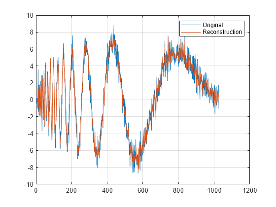
Obtain the single-level DWT of the noisy Doppler signal using the "sym4" wavelet.
load noisdopp;
[cA,cD] = dwt(noisdopp,"sym4");
Reconstruct a smoothed version of the signal using the approximation coefficients. Plot and compare with the original signal.
xrec = idwt(cA,zeros(size(cA)),"sym4");
plot(noisdopp)
hold on
grid on
plot(xrec)
legend("Original","Reconstruction")
hold off
Obtain the single-level DWT of a noisy Doppler signal using the wavelet (highpass) and scaling (lowpass) filters.
load noisdopp
[LoD,HiD] = wfilters("bior3.5","d");
[cA,cD] = dwt(noisdopp,LoD,HiD);
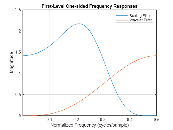
Create a DWT filter bank that can be applied to the noisy Doppler signal using the same wavelet. Obtain the highpass and lowpass filters from the filter bank.
len = length(noisdopp);
fb = dwtfilterbank("SignalLength",len,"Wavelet","bior3.5");
[lo,hi] = filters(fb);
For the bior3.5 wavelet, lo and hi are 12-by-2 matrices. lo are the lowpass filters, and hi are the highpass filters. The first columns of lo and hi are used for analysis and the second columns are used for synthesis. Compare the first column of lo and hi with LoD and HiD respectively. Confirm they are equal.
disp("Lowpass Analysis Filters")Lowpass Analysis Filters
[lo(:,1) LoD']
ans = 12×2

   -0.0138   -0.0138
    0.0414    0.0414
    0.0525    0.0525
   -0.2679   -0.2679
   -0.0718   -0.0718
    0.9667    0.9667
    0.9667    0.9667
   -0.0718   -0.0718
   -0.2679   -0.2679
    0.0525    0.0525
    0.0414    0.0414
   -0.0138   -0.0138
disp("Highpass Analysis Filters")Highpass Analysis Filters
[hi(:,1) HiD']
ans = 12×2

         0         0
         0         0
         0         0
         0         0
   -0.1768   -0.1768
    0.5303    0.5303
   -0.5303   -0.5303
    0.1768    0.1768
         0         0
         0         0
         0         0
         0         0
Plot the one-sided magnitude frequency responses of the first-level wavelet and scaling filters.
[psidft,f,phidft] = freqz(fb);
level = 1;
plot(f(len/2+1:end),abs(phidft(level,len/2+1:end)))
hold on
plot(f(len/2+1:end),abs(psidft(level,len/2+1:end)))
grid on
hold off
legend("Scaling Filter","Wavelet Filter")
title("First-Level One-sided Frequency Responses")
xlabel("Normalized Frequency (cycles/sample)")
ylabel("Magnitude")
Refer to GPU Computing Requirements (Parallel Computing Toolbox) to see what GPUs are supported.
Load the noisy Doppler signal. Put the signal on the GPU using gpuArray. Save the current extension mode.
load noisdopp
noisdoppg = gpuArray(noisdopp);
origMode = dwtmode("status","nodisp");
Use dwtmode to change the extension mode to zero-padding. Obtain the single-level discrete wavelet transform of the signal on the GPU using the db2 wavelet.
dwtmode("zpd","nodisp")
[cA,cD] = dwt(noisdoppg,"db2");
The current extension mode zpd is not supported for gpuArray input. Therefore, the DWT is instead performed using the sym extension mode. Confirm this by taking the DWT of noisdoppg with the extension mode set to sym and compare with the previous result.
[cAsym,cDsym] = dwt(noisdoppg,"db2","mode","sym");
[max(abs(cA-cAsym)) max(abs(cD-cDsym))]
ans =

     0     0
An unsupported extension mode specified as an input argument is converted to "sym". Confirm that taking the DWT of noisdoppg with "mode" set to an unsupported mode also defaults to the sym extension mode.
[cA,cD] = dwt(noisdoppg,"db2","mode","spd");
[max(abs(cA-cAsym)) max(abs(cD-cDsym))]
ans =

     0     0
Change the current extension mode to periodic. Obtain the single-level discrete wavelet transform of the signal on the GPU using the db2 wavelet.
dwtmode("per","nodisp")
[cA,cD] = dwt(noisdoppg,"db2");
Confirm the current extension mode per is supported for gpuArray input.
[cAper,cDper] = dwt(noisdopp,"db2","mode","per");
[max(abs(cA-cAper)) max(abs(cD-cDper))]
ans =

     0     0
Restore the extension mode to the original setting.
dwtmode(origMode,"nodisp")Input Arguments
Output Arguments
Algorithms
Starting from a signal s of length N, two sets of
coefficients are computed: approximation coefficients
cA1, and detail coefficients
cD1. Convolving s with the scaling
filter LoD, followed by dyadic decimation, yields the approximation
coefficients. Similarly, convolving s with the wavelet filter
HiD, followed by dyadic decimation, yields the detail coefficients.

where
 — Convolve with filter X
— Downsample (keep the even-indexed elements)
The length of each filter is equal to 2n. If N = length(s), the signals F and G are of length N + 2n −1 and the coefficients cA1 and cD1 are of length floor.
To deal with signal-end effects resulting from a convolution-based algorithm, a global
variable managed by dwtmode defines the kind of signal extension mode
used. The possible options include zero-padding and symmetric extension, which is the default
mode.
Note
For the same input, the dwt function and the DWT block in the
DSP System Toolbox™ do not produce the same results. The DWT block is designed for real-time
implementation while Wavelet Toolbox™ software is designed for analysis, so the products handle boundary conditions and
filter states differently.
To make the dwt function output match the DWT block output, set the
function boundary condition to zero-padding by typing dwtmode("zpd") at the
MATLAB® command prompt. To match the latency of the DWT block, which is implemented using
FIR filters, add zeros to the input of the dwt function. The number of
zeros you add must be equal to half the filter length.
References
[1] Daubechies, I. Ten Lectures on Wavelets. CBMS-NSF Regional Conference Series in Applied Mathematics. Philadelphia, PA: Society for Industrial and Applied Mathematics, 1992.
[2] Mallat, S. G. “A Theory for Multiresolution Signal Decomposition: The Wavelet Representation.” IEEE Transactions on Pattern Analysis and Machine Intelligence. Vol. 11, Issue 7, July 1989, pp. 674–693.
[3] Meyer, Y. Wavelets and Operators. Translated by D. H. Salinger. Cambridge, UK: Cambridge University Press, 1995.
Extended Capabilities
Version History
Introduced before R2006aSee Also
wavedec | idwt | dwtmode | waveinfo | dwtfilterbank