wavedec
Multilevel 1-D discrete wavelet transform
Description
Examples
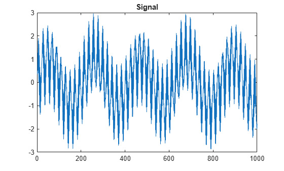
Load and plot a one-dimensional signal.
load sumsin
plot(sumsin)
title("Signal")
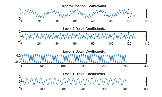
Perform a 3-level wavelet decomposition of the signal using the order 2 Daubechies wavelet. Extract the coarse scale approximation coefficients and the detail coefficients from the decomposition.
[c,l] = wavedec(sumsin,3,"db2");
approx = appcoef(c,l,"db2");
[cd1,cd2,cd3] = detcoef(c,l,[1 2 3]);
Plot the coefficients.
tiledlayout(4,1)
nexttile
plot(approx)
title("Approximation Coefficients")
nexttile
plot(cd3)
title("Level 3 Detail Coefficients")
nexttile
plot(cd2)
title("Level 2 Detail Coefficients")
nexttile
plot(cd1)
title("Level 1 Detail Coefficients")
Refer to GPU Computing Requirements (Parallel Computing Toolbox) to see what GPUs are supported.
Load the noisy Doppler signal. Put the signal on the GPU using gpuArray. Save the current global DWT extension mode.
load noisdopp
noisdoppg = gpuArray(noisdopp);
origMode = dwtmode("status","nodisp");
Obtain the three-level DWT of the signal on the GPU using the db4 wavelet. Even though the zpd extension mode is not supported for gpuArray input, specify it. The wavedec function instead uses the sym extension mode.
[czpd,lzpd] = wavedec(noisdoppg,3,"db4",Mode="zpd");
Confirm that the wavedec function did use the sym extension mode. Set the global extension mode to sym and obtain the three-level DWT of noisdoppg without specifying an extension mode. Confirm this result equals the previous result.
dwtmode("sym","nodisp")
[csym,lsym] = wavedec(noisdoppg,3,"db4");
[max(abs(czpd-csym)) max(abs(lzpd-lsym))]
ans =

     0     0
Obtain the three-level DWT of noisdoppg using the per extension mode, which is supported for gpuArray input. Confirm this result is different from the sym result.
[cper,lper] = wavedec(noisdoppg,3,"db4",Mode="per");
[length(csym) ; length(cper)]
ans = 2×1

        1044
        1024
[lsym ; lper]
ans =

         134         134         261         515        1024
         128         128         256         512        1024
Restore the global extension mode to the original setting.
dwtmode(origMode,"nodisp")This example shows how, starting with a multilevel 1-D discrete wavelet decomposition of a signal, you can obtain projections of the signal onto wavelet subspaces at successive scales and a scaling subspace. These projections are at the same time scale as the original signal. In other words, you can obtain a multiresolution analysis (MRA) based on the decimated discrete wavelet transform (DWT). You can recover the signal by summing the projections. For more information, see Practical Introduction to Multiresolution Analysis.
Load and plot a signal.
load noissin
plot(noissin)
title("Original Signal")

Use the wavedec function to obtain the discrete wavelet decomposition of the signal down to level 3 using the db4 wavelet.
level = 3;
wv = "db4";
[C,L] = wavedec(noissin,level,wv);
Preallocate a matrix to save the MRA. The number of rows is one more than the level of decomposition, and the number of columns equals the length of the signal.
mra = zeros(level+1,numel(noissin));
Use the wrcoef function to obtain the projections of the signal onto the three wavelet (detail) subspaces. Then obtain the projection onto the final scaling (coarse or approximation) subspace.
for k=1:level
    mra(k,:) = wrcoef("d",C,L,wv,k);
end
mra(end,:) = wrcoef("a",C,L,wv,level);
Confirm the sum along the rows of the MRA equals the original signal.
mraSum = sum(mra,1);
max(abs(mraSum-noissin))
ans =
1.6591e-12
Plot the MRA.
tiledlayout(level+1,1)
for k=1:level
    nexttile
    plot(mra(k,:))
    title("Projection Onto Detail Subspace "+num2str(k))
end
nexttile
plot(mra(end,:))
title("Projection Onto Approximation Subspace")

Input Arguments
Output Arguments
Wavelet decomposition vector, returned as a vector.
Data Types: single | double
Bookkeeping vector, returned as a vector of positive integers. The vector contains the number of coefficients by level and the length of the original signal.
The bookkeeping vector is used to parse the coefficients in the wavelet
decomposition vector c by level. The decomposition
vector and bookkeeping vector are organized as in this level-3 decomposition diagram.
Data Types: single | double
Algorithms
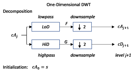
Given a signal s of length N, the DWT consists
of at most log2
N steps. Starting from s, the first step produces
two sets of coefficients: approximation coefficients
cA1 and detail coefficients
cD1. Convolving s
with the lowpass filter LoD and the highpass filter
HiD, followed by dyadic decimation (downsampling by 2), results
in the approximation and detail coefficients respectively.

where
 — Convolve with filter X
— Downsample (keep the even-indexed elements)
The length of each filter is equal to 2n. If N = length(s), the signals F and G are of length N + 2n −1 and the coefficients cA1 and cD1 are of length
floor.
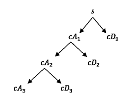
The next step splits the approximation coefficients cA1 in two parts using the same scheme, replacing s by cA1, and producing cA2 and cD2, and so on.
The wavelet decomposition of the signal s analyzed at level j has the following structure: [cAj, cDj, ..., cD1].
This structure contains, for j = 3, the terminal nodes of the following tree:
References
[1] Daubechies, I. Ten Lectures on Wavelets, CBMS-NSF Regional Conference Series in Applied Mathematics. Philadelphia, PA: SIAM Ed, 1992.
[2] Mallat, S.G. “A Theory for Multiresolution Signal Decomposition: The Wavelet Representation.” IEEE Transactions on Pattern Analysis and Machine Intelligence 11, no. 7 (July 1989): 674–93. https://doi.org/10.1109/34.192463.
[3] Meyer, Y. Wavelets and Operators. Translated by D. H. Salinger. Cambridge, UK: Cambridge University Press, 1995.