Create Plot
Interactively create linear analysis response plots in the Live Editor
Since R2022b
Description
The Create Plot Live Editor task lets you
interactively create time-domain and frequency-domain analysis plots for dynamic system models
in your MATLAB® workspace. This page describes a subset of the functionality available in the
Create Plot
live task — the subset available when you select Control Toolbox
Plots in the Filter by Category menu. For more
information about the task in general, see the Create Plot
Live Editor task reference page.
For more information about Live Editor tasks generally, see Add Interactive Tasks to a Live Script.
Supported plots
The Create Plot Live Editor task supports the following linear analysis response plots:
Open the Task
To add the Create Plot task to a live script in the MATLAB Live Editor:
On the Live Editor tab, click Task and select the Create Plot icon
 .
.In a code block in the live script, type a relevant keyword, such as
bode,step,pzplot, orimpulse. Select Create Plot from the suggested command completions. When you add the task using this method, then MATLAB automatically selects the corresponding chart type in the Select visualization section of the task.
Examples
Use the Create Plot task in the Live Editor to interactively create and visualize different linear analysis plots. You can also use an options object from your MATLAB® workspace to customize your plot. Open this example to see a preconfigured script containing the Create Plot task to create a Bode plot.
For this example, consider the following SISO state-space model:
Create the SISO state-space model defined by the following state-space matrices:
A = [-1.5,-2;1,0];
B = [0.5;0];
C = [0,1];
D = 0;
sys = ss(A,B,C,D);
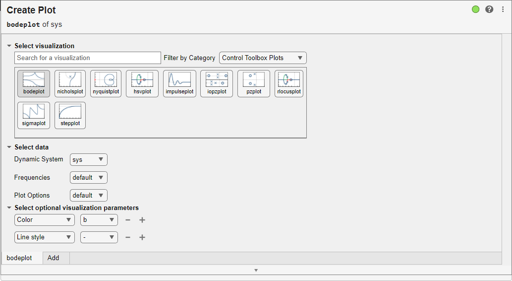
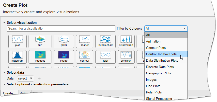
To create a Bode plot of sys, open the Create Plot task in the Live Editor. On the Live Editor tab, select Task > Create Plot. In the task, select Control Toolbox Plots from the Filter by Category dropdown menu. You can also directly search for the plot type by typing in the plot name in the Select visualization field.
Next, select bodeplot from the available plots. If you do not have a supported model type in your MATLAB workspace, then the respective plot type will not be available.

Use the Dynamic System dropdown menu to pick the appropriate model from your MATLAB workspace. You can use the Frequencies dropdown menu to specify a vector of frequencies. You can also customize your plot by using a predefined options object. For more information, see bodeplot.
For this example, pick sys and leave the other options as default.


You can also select the color, line style and marker symbol for the plot using the Select optional visualization parameters menu. You can click ![]() to add more visualization parameters. For this example, change the line color to green.
to add more visualization parameters. For this example, change the line color to green.


To see the code that this task generates, expand the task display by clicking ![]() Show code at the bottom of the task parameter area.
Show code at the bottom of the task parameter area.

You can also overlay multiple visualizations on the same plot axis. For more information and examples, see the Create Plot task reference page.
Parameters
Version History
Introduced in R2022b
See Also
Functions
bodeplot|stepplot|rlocusplot|impulseplot|nicholsplot|nyquistplot|pzplot|hsvplot|iopzplot|sigmaplot|bodeoptions|nicholsoptions|hsvoptions|nyquistoptions|pzoptions|sigmaoptions|timeoptions