Main Content

legendre

Associated Legendre functions

Description

P = legendre(n,X) computes the associated Legendre functions of degree n and order m = 0, 1, ..., n evaluated for each element in X.

example

P = legendre(n,X,normalization) computes normalized versions of the associated Legendre functions. normalization can be 'unnorm' (default), 'sch', or 'norm'.

example

Examples

collapse all

Use the legendre function to operate on a vector and then examine the format of the output.

Calculate the second-degree Legendre function values of a vector.

deg = 2;
x = 0:0.1:0.2;
P = legendre(deg,x)
P = 3×3

   -0.5000   -0.4850   -0.4400
         0   -0.2985   -0.5879
    3.0000    2.9700    2.8800

The format of the output is such that:

  • Each row contains the function value for different values of m (the order of the associated Legendre function)

  • Each column contains the function value for a different value of x

x = 0x = 0.1x = 0.2m = 0P20(0)P20(0.1)P20(0.2)m = 1P21(0)P21(0.1)P21(0.2)m = 2P22(0)P22(0.1)P22(0.2)

The equation for the second-degree associated Legendre function P2m is

P2m(x)=(-1)m(1-x2)m/2dmdxm[12(3x2-1)].

Therefore, the value of P20(0) is

P20(0)=[12(3x2-1)]|x=0=-12.

This result agrees with P(1,1) = -0.5000.

Calculate the associated Legendre function values with several normalizations.

Calculate the first-degree, unnormalized Legendre function values P1m. The first row of values corresponds to m=0, and the second row to m=1.

x = 0:0.2:1;
n = 1;
P_unnorm = legendre(n,x)
P_unnorm = 2×6

         0    0.2000    0.4000    0.6000    0.8000    1.0000
   -1.0000   -0.9798   -0.9165   -0.8000   -0.6000         0

Next, compute the Schmidt seminormalized function values. Compared to the unnormalized values, the Schmidt form differs when m>0 by the scaling

(-1)m2(n-m)!(n+m)!.

For the first row, the two normalizations are the same, since m=0. For the second row, the scaling constant multiplying each value is -1.

P_sch = legendre(n,x,'sch')
P_sch = 2×6

         0    0.2000    0.4000    0.6000    0.8000    1.0000
    1.0000    0.9798    0.9165    0.8000    0.6000         0

C1 = (-1) * sqrt(2*factorial(0)/factorial(2))
C1 = 
-1

Lastly, compute the fully normalized function values. Compared to the unnormalized values, the fully normalized form differs by the scaling factor

(-1)m(n+12)(n-m)!(n+m)!.

This scaling factor applies for all values of m, so the first and second rows have different scaling factors.

P_norm = legendre(n,x,'norm')
P_norm = 2×6

         0    0.2449    0.4899    0.7348    0.9798    1.2247
    0.8660    0.8485    0.7937    0.6928    0.5196         0

Cm0 = sqrt((3/2))
Cm0 = 
1.2247
Cm1 = (-1) * sqrt((3/2)/2)
Cm1 = 
-0.8660

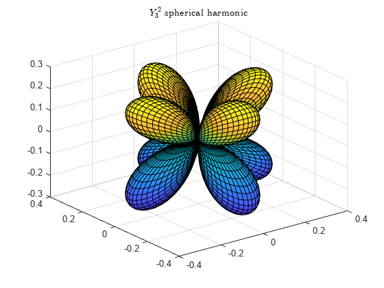
Spherical harmonics arise in the solution to Laplace's equation and are used to represent functions defined on the surface of a sphere. Use legendre to compute and visualize the spherical harmonic for Y32.

The equation for spherical harmonics includes a term for the Legendre function, as well as a complex exponential:

Ylm(θ,ϕ)=(2l+1)(l-m)!4π(l+m)!Plm(cosθ)eimϕ,-lml.

First, create a grid of values to represent all combinations of 0θπ (colatitude angle) and 0ϕ2π (azimuthal angle). Here, the colatitude θ ranges from 0 at the North Pole, to π/2 at the Equator, and to π at the South Pole.

dx = pi/60;
col = 0:dx:pi;
az = 0:dx:2*pi;
[phi,theta] = meshgrid(az,col);

Calculate Plm(cosθ) on the grid for l=3.

l = 3;
Plm = legendre(l,cos(theta));

Since legendre computes the answer for all values of m, Plm contains some extra function values. Extract the values for m=2 and discard the rest. Use the reshape function to orient the results as a matrix with the same size as phi and theta.

m = 2;
if l ~= 0
    Plm = reshape(Plm(m+1,:,:),size(phi));
end

Calculate the spherical harmonic values for Y32.

a = (2*l+1)*factorial(l-m);
b = 4*pi*factorial(l+m);
C = sqrt(a/b);
Ylm = C .*Plm .*exp(1i*m*phi);

Convert the spherical coordinates to Cartesian coordinates. Here, π/2-θ becomes the latitude angle that ranges from π/2 at the North Pole, to 0 at the Equator, and to -π/2 at the South Pole. Plot the spherical harmonic for Y32 using both the positive and negative real values.

[Xm,Ym,Zm] = sph2cart(phi, pi/2-theta, abs(real(Ylm)));
surf(Xm,Ym,Zm)
title('$Y_3^2$ spherical harmonic','interpreter','latex')

Figure contains an axes object. The axes object with title YSubScript 3 SuperScript 2 baseline spherical harmonic contains an object of type surface.

Input Arguments

collapse all

Degree of Legendre function, specified as a positive integer. For a specified degree, legendre computes Pnm(x) for all orders m from m = 0 to m = n.

Example: legendre(2,X)

Input values, specified as a scalar, vector, matrix, or multidimensional array of real values in the range [-1,1]. For example, with spherical harmonics it is common to use X = cos(theta) as the input values to compute Pnm(cosθ).

Example: legendre(2,cos(theta))

Data Types: single | double

Normalization type, specified as one of these values.

Example: legendre(n,X,'sch')

Output Arguments

collapse all

Associated Legendre function values, returned as a scalar, vector, matrix, or multidimensional array. The normalization of P depends on the value of normalization.

The size of P depends on the size of X:

  • If X is a vector, then P is a matrix of size (n+1)-by-length(X). The P(m+1,i) entry is the associated Legendre function of degree n and order m evaluated at X(i).

  • In general, P has one more dimension than X and each element P(m+1,i,j,k,...) contains the associated Legendre function of degree n and order m evaluated at X(i,j,k,...).

Limitations

The values of the unnormalized associated Legendre function overflow the range of double-precision numbers for n > 150 and the range of single-precision numbers for n > 28. This overflow results in Inf and NaN values. For orders larger than these thresholds, consider using the 'sch' or 'norm' normalizations instead.

More About

collapse all

Associated Legendre Functions

The associated Legendre functions y=Pnm(x) are solutions to the general Legendre differential equation

(1x2)d2ydx22xdydx+[n(n+1)m21x2]y=0.

n is the integer degree and m is the integer order of the associated Legendre function, such that 0mn.

The associated Legendre functions Pnm(x) are the most general solutions to this equation given by

Pnm(x)=(1)m(1x2)m/2dmdxmPn(x).

They are defined in terms of derivatives of the Legendre polynomials Pn(x), which are a subset of the solutions given by

Pn(x)=12nn!dndxn(x21)n.

The first few Legendre polynomials are

Value of nPn(x)
0P0(x)=1
1P1(x)=x
2P2(x)=12(3x21)

Schmidt Seminormalized Associated Legendre Functions

The Schmidt seminormalized associated Legendre functions are related to the unnormalized associated Legendre functions Pnm(x) by

Pn(x) for m=0,Snm(x)=(1)m2(nm)!(n+m)!Pnm(x) for m>0.

Fully Normalized Associated Legendre Functions

The fully normalized associated Legendre functions are normalized such that

11[Nnm(x)]2dx=1.

The normalized functions are related to the unnormalized associated Legendre functions Pnm(x) by

Nnm(x)=(1)m(n+12)(nm)!(n+m)!Pnm(x).

Algorithms

legendre uses a three-term backward recursion relationship in m. This recursion is on a version of the Schmidt seminormalized associated Legendre functions Qnm(x), which are complex spherical harmonics. These functions are related to the standard Abramowitz and Stegun [1] functions Pnm(x) by

Pnm(x)=(n+m)!(nm)!Qnm(x).

They are related to the Schmidt form by

m=0:Snm(x)=Qn0(x)m>0:Snm(x)=(1)m2Qnm(x).

References

[1] Abramowitz, M. and I. A. Stegun, Handbook of Mathematical Functions, Dover Publications, 1965, Ch.8.

[2] Jacobs, J. A., Geomagnetism, Academic Press, 1987, Ch.4.
Extended Capabilities

Version History

Introduced before R2006a

Go to top of page