odeSensitivity

ODE sensitivity analysis

Since R2024a

Description

Use odeSensitivity objects to perform sensitivity analysis on a system of ordinary differential equations (ODEs) or differential algebraic equations (DAEs). Sensitivity analysis examines how changes in the values of parameters in the differential equations affect the calculated solutions. If an equation is sensitive to the value of a particular parameter, then small changes in the parameter value can produce large changes in the solution.

Create an ode object to represent the ODE or DAE problem, and specify an odeSensitivity object as the value of the Sensitivity property to perform sensitivity analysis.

Creation

Syntax

S = odeSensitivity

S = odeSensitivity(Name=Value)

Description

S = odeSensitivity creates an odeSensitivity object with empty properties.

S = odeSensitivity(Name=Value) specifies one or more property values using name-value arguments. For example, you can specify the equation parameters to include in the sensitivity analysis by using the ParameterIndices property.

Properties

ParameterIndices — Parameter indices for sensitivity analysis

scalar index | vector of indices

Parameter indices for sensitivity analysis, specified as a scalar index or vector of indices. ParameterIndices contains indices into the numeric Parameters property of the ode object to specify which parameters to include in the sensitivity analysis.

If you do not specify a value for ParameterIndices, then the ode object performs sensitivity analysis on all parameters.

Example: S = odeSensitivity(ParameterIndices=1:2) specifies that the first and second parameters are used for sensitivity analysis.

InitialValue — Initial sensitivity of solution

matrix

Initial sensitivity of solution, specified as a matrix. The matrix has one row for each equation in the system, and one column for each sensitivity parameter as defined by the ParameterIndices property. Each (i,j) value in the matrix specifies the initial sensitivity of equation i with respect to sensitivity parameter j.

If you do not specify a value for InitialValue, then the ode object uses a matrix of zeros.

Example: S = odeSensitivity(InitialValue=M) specifies a matrix M of initial sensitivities.

InitialSlope — Initial slope for DAE problems

vector

Initial slope for DAE problems, specified as a vector. Use this property with the idas solver when solving DAEs. The vector specifies the initial slope ds/dt for each sensitivity parameter as defined by the ParameterIndices property.

If the specified initial slopes are not consistent with the InitialTime, InitialValue, and MassMatrix properties of the ode object, then the solver treats the slopes as guesses and attempts to compute consistent values for the initial slopes that are close to the guesses before continuing to solve the problem.

If you do not specify a value for InitialSlope, then the ode object uses a vector of zeros.

Example: S = odeSensitivity(InitialSlope=[0.1 0.2]) specifies initial slopes for two sensitivity parameters.

Jacobian — Jacobian matrix with respect to parameters

odeJacobian object | matrix | function handle

Jacobian matrix with respect to parameters, specified as an odeJacobian object, matrix, or handle to a function that evaluates the Jacobian. The Jacobian is a matrix of partial derivatives of the functions that define the system of differential equations with respect to one or more parameters defined in the Parameters property of the ode object. The Jacobian matrix has one row for each equation in the system and one column for each sensitivity parameter as defined by the ParameterIndices property.

$$J=\frac{\partial f}{\partial p}=\left[\begin{array}{ccc}\frac{\partial f_1}{\partial p_1}& \frac{\partial f_1}{\partial p_2}& \cdots \\ \frac{\partial f_2}{\partial p_1}& \frac{\partial f_2}{\partial p_2}& \cdots \\ ⋮& ⋮& \end{array}\right]$$

The Jacobian is used for all sensitivity analyses, regardless of solver choice. If you do not provide the Jacobian, then the ODE solver approximates it numerically using finite differences.

For large systems of equations where it is not feasible to provide the entire analytic Jacobian, you can specify the sparsity pattern of the Jacobian matrix instead. The solver uses the sparsity pattern to calculate a sparse Jacobian.

You can specify the value of the Jacobian property as:

• An odeJacobian object, which can represent either the Jacobian matrix or its sparsity pattern.

• A constant matrix with calculated values for the Jacobian elements.

• A handle to a function that computes the matrix elements and that accepts two input arguments, dfdp = Fjac(t,y). To give the function access to parameter values in the Parameters property, specify a third input argument in the function definition, dfdp = Fjac(t,y,p).

If you specify a matrix or function handle, then MATLAB^® converts it to an odeJacobian object.

Example: S = odeSensitivity(Jacobian=@Fjac) specifies the function Fjac that evaluates the Jacobian matrix.

Example: S = odeSensitivity(Jacobian=[0 1; -2 1]) specifies a constant Jacobian matrix.

Example: S = odeSensitivity(Jacobian=odeJacobian(SparsityPattern=S)) specifies the Jacobian sparsity pattern using sparse matrix S.

Examples

Examine Parameter Sensitivity

Solve an ODE system with two equations and two parameters, and perform sensitivity analysis on the parameters.

Create an ode object to represent this system of equations.

$$\begin{array}{l}\frac{{\mathrm{dy}}_1}{\mathrm{dt}}={\mathit{p}}_1{\mathit{y}}_1-{\mathit{y}}_2\\ \frac{{\mathrm{dy}}_2}{\mathrm{dt}}={-\mathit{p}}_2{\mathit{y}}_2\end{array}$$

Specify the initial conditions as ${\mathit{y}}_1\left(0\right)=2$ and ${\mathit{y}}_2\left(0\right)=3$, and parameter values of ${\mathit{p}}_1=0.05$ and ${\mathit{p}}_2=1.5$. To enable sensitivity analysis of the parameters, set the Sensitivity property of the ode object to an odeSensitivity object.

p = [0.05 1.5];
F = ode(ODEFcn=@(t,y,p) [p(1)*y(1)-y(2); -p(2)*y(2)], ...
        InitialValue=[2 3], ...
        Parameters=p, ...
        Sensitivity=odeSensitivity)

F = 
  ode with properties:

   Problem definition
               ODEFcn: @(t,y,p)[p(1)*y(1)-y(2);-p(2)*y(2)]
           Parameters: [0.0500 1.5000]
          InitialTime: 0
         InitialValue: [2 3]
          Sensitivity: [1x1 odeSensitivity]
         EquationType: standard

   Solver properties
    AbsoluteTolerance: 1.0000e-06
    RelativeTolerance: 1.0000e-03
               Solver: auto
       SelectedSolver: cvodesnonstiff

  Show all properties

Because the equations are nonstiff and sensitivity analysis is enabled, the ode object automatically chooses the cvodesnonstiff solver for this problem.

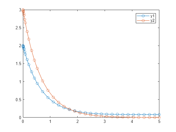
Solve the ODE over the time interval [0 5], and plot the solution for each component.

S = solve(F,0,5)

S = 
  ODEResults with properties:

           Time: [0 2.9540e-09 2.9543e-05 2.2465e-04 4.1976e-04 0.0024 0.0080 0.0137 0.0245 0.0353 0.0611 0.0869 0.1499 0.2129 0.3169 0.4208 0.5248 0.7204 0.9161 1.1118 1.3075 1.5031 1.6988 1.8945 2.0901 2.2858 2.4815 2.6772 2.8728 ... ] (1x40 double)
       Solution: [2x40 double]
    Sensitivity: [2x2x40 double]

plot(S.Time,S.Solution(1,:),"-o",S.Time,S.Solution(2,:),"-o")
legend("y1","y2")

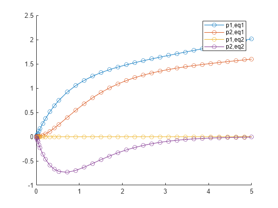
The values in S.Sensitivity are partial derivatives of the equations with respect to the parameters. To examine the effects of the parameter values during the integration, plot the sensitivity values.

figure
hold on
plot(S.Time,squeeze(S.Sensitivity(1,1,:)),"-o")
plot(S.Time,squeeze(S.Sensitivity(1,2,:)),"-o")
plot(S.Time,squeeze(S.Sensitivity(2,1,:)),"-o")
plot(S.Time,squeeze(S.Sensitivity(2,2,:)),"-o")
legend("p1,eq1","p2,eq1","p1,eq2","p2,eq2")
hold off

Version History

Introduced in R2024a