Load Predefined Multiagent Environments

Reinforcement Learning Toolbox™ software provides two predefined environments in which two agents interact with each other to collaboratively push a larger object outside a circular boundary. You can use these environments to learn how to apply reinforcement learning to multiagent systems, to test your own agents, or as a starting point for developing your own multiagent environment.

To create your own custom multiagent environments instead, use rlTurnBasedFunctionEnv and rlMultiAgentFunctionEnv. For more information on training multiagent environments, see Multiagent Training.

The two predefined multiagent environments are derived by discretizing the dynamics of the same physical system as they rely on the same internal function to calculate the dynamics. The environments have the same inputs, outputs, internal states, and parameters, but one is a MATLAB^® environment and the other is a Simulink^® environment. When designing your own multiagent environment, you can use as a starting point the implementation that makes most sense for your application.

Environment	Implementation
Pusher	MATLAB
PusherModel	Simulink

In these environments, the state and observations belong to continuous numerical vector spaces, while the action of each agent can belong to either a continuous or finite set. Specifically, each of these predefined environments is available in two versions:

• In the discrete version both agents have a discrete action space.

• In the continuous version both agents have a continuous action space.

To load the predefined multiagent environments, use the rlPredefinedEnv function.

MATLAB Pusher Environment

A MATLAB pusher environment is a predefined MATLAB environment featuring two agents, referred to as agents A and B. Each agent exerts a planar force on a two-dimensional disk that as a result can slide on the plane, according to Newton's laws of motion. The two disks guided by the agents can collide with each other and with a third disk. The goal of the agents is to push the third disk completely outside a circular boundary using minimal control effort.

This environment is equivalent to the predefined Simulink PusherModel environment, with some differences in the number of accessible properties, and the availability of the plot function. You can use the implementation that you are most comfortable with as a starting point when designing and developing your own multiagent environment.

There are two variants of the predefined MATLAB pusher environment, which differ by the agent action space:

• Discrete — The agent can apply a force which is quantized along the horizontal and vertical dimensions in five points consisting of -MaxForce, -MaxForce/2, 0, MaxForce/2, and MaxForce.

• Continuous — The agent can apply any torque within the range [-MaxForce,MaxForce].

Here, MaxForce is an environment property that you can change using dot notation. For more information, see Environment Properties.

You can set the UseContinuousAction property of this environment to establish whether each agent must have a continuous or discrete action space. For example, you can set the action spaces of the two agents differently, so that one agent has a discrete action space and the other agent has a continuous action space.

To create a predefined MATLAB pusher environment, use rlPredefinedEnv as follows, depending on the desired action space:

• Discrete action space:

  env = rlPredefinedEnv("Pusher-Discrete")

  env = 
  
    PusherEnvironment with properties:
  
                            Width: 20
                           Height: 20
                         MaxForce: 5
                       TaskRadius: 8
                   ParticleRadius: [0.2500 0.2500 0.7500]
                     ParticleMass: [1 1 10]
       VelocityDampingCoefficient: [0.1000 0.1000 10]
      ContactStiffnessCoefficient: 1000
              UseContinuousAction: [0 0]
                               Ts: 0.0200

• Continuous action space:

  env = rlPredefinedEnv("Pusher-Continuous")

  env = 
  
    PusherEnvironment with properties:
  
                            Width: 20
                           Height: 20
                         MaxForce: 5
                       TaskRadius: 8
                   ParticleRadius: [0.2500 0.2500 0.7500]
                     ParticleMass: [1 1 10]
       VelocityDampingCoefficient: [0.1000 0.1000 10]
      ContactStiffnessCoefficient: 1000
              UseContinuousAction: [1 1]
                               Ts: 0.0200

Environment Visualization

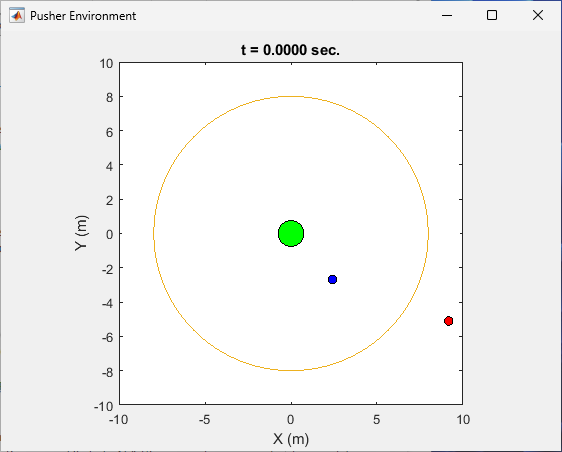
You can visualize the predefined MATLAB pusher environment using the plot function. The green circle at the origin represents disk C, which the agents have to move out of the task boundary, represented by the orange circle. The smaller blue and red circles represent the disks guided by agents A and B, respectively.

plot(env)

To visualize the environment during training, call plot before training and keep the visualization figure open.

Note

While visualizing the environment during training might often be insightful, doing so tends to increase training time. For faster training, keep the environment plot closed during training.

Environment Properties

All the environment properties listed in this table are writable. You can change them to customize the pusher environment to your needs.

Property	Description	Default
Width	Width in meters of the rectangular region in which the disks must stay. Disks bounce off the boundary of this region when attempting to move through it.	20
Height	Height in meters of the rectangular region in the which disks move. Disks bounce off the boundary of this region when attempting to move through it.	20
MaxForce	Maximum force in newtons that an agent can apply to its disk	5
TaskRadius	Radius in meters of the circular boundary out of which the agents have to push the third disk	8
ParticleRadius	Radii of the disks in meters, specified as [rA,rB,rC], where rA and rB are the radii of the disks guided by agents A and B, respectively, and rC is the radii of the third disk.	[0.25 0.25 0.75]
ParticleMass	Masses of the disks in kilograms, specified as [mA,mB,mC], where mA and mB are the masses of the disks guided by agents A and B, respectively, and mC is the mass of the third disk.	[1 1 10]
VelocityDampingCoefficient	Damping on disks motion (viscous friction), in newtons per second over meters, specified as [dA,dB,dc], where dC and dB are the damping coefficients for the disks guided by agents A and B, respectively, and dC is the damping coefficient for the third disk.	[0.1 0.1 10]
ContactStiffnessCoefficient	Coefficient for computing contact forces (contact forces are modeled as static spring forces). For more information, see Dynamics.	1000
UseContinuousAction	Option to enable continuous action space for agents A and B, respectively, specified as a vector containing two logical values.	[0 0]
Ts	Sample time in seconds. The software uses the sample time to discretize the dynamics of the underlying continuous-time system. The discrete-time dynamics is then used to calculate the next state as a function of the current state and of the applied action.	0.05

Dynamics

The two agents A and B exert forces u_A and u_B on their respective disks. Per Newton's second law, the disks, which are subjected to viscous friction, move on a planar horizontal surface. The disks guided by the agents can collide with each other, with a third disk initially positioned at the origin, and with the boundary of the larger rectangular area within which all three disks are confined. Collisions are modeled as a mass-spring system. These equations represent the continuous-time dynamics of the environment.

$$\begin{array}{l}{m}_A{\ddot{p}}_A+d_A{\dot{p}}_A=u_A+F_A\left(p_A,p_B,p_C\right)\\ m_B{\ddot{p}}_B+d_B{\dot{p}}_B=u_B+F_B\left(p_A,p_B,p_C\right)\\ m_C{\ddot{p}}_C+d_C{\dot{p}}_C=F_C\left(p_A,p_B,p_C\right)\end{array}$$

Here, using an index i to denote subscripts A, B, and C:

• m_i are the masses of the three disks.

• p_i are the positions of the three disks on the plane. Each position has scalar components x_i (positive-right) and y_i (positive-up). Each dot above p_i denotes a derivative with respect to time.

• d_i are the damping coefficients used to calculate the viscous friction force on the three disks.

• F_i is the force exerted on the disk i as a consequence of the collision with another disk or with the rectangular boundary wall.

Specifically,

• No collision — When p_i is within the rectangular boundary and D_ij is greater than R_ij, then F_i is zero.

• Collision with another disk — when p_i is within the rectangular boundary and D_ij is less than R_ij, then F_i is equal to –k_i multiplied by the transition distance D_ij–R_ij.

• Collision with a wall — when p_i is outside the rectangular boundary, then F_i is equal to –k_i multiplied by the distance from the disk surface to the wall: p_i+r_i–W.

The software then uses a Runge-Kutta integration method to obtain the discrete-time dynamics of the environment.

Actions

In the predefined MATLAB pusher environment, each agent uses its own action channel. Each action channel carries a two-element vector containing the (normalized) forces applied by the agent to its disk in the x (positive-right) and y (positive-up) directions. The action space is specified as follows:

• Discrete action spaces — by default, the specification for the action channel of each agent is an rlFiniteSetSpec object.

  actInfo = getActionInfo(env)

    actInfo =
  
    1×2 cell array
  
      {1×1 rl.util.rlFiniteSetSpec}    {1×1 rl.util.rlFiniteSetSpec}
  
  

  If you set the UseContinuousAction property of the environment so that an agent uses a continuous action space, then the action channel of that agent is an rlNumericSpec object.

  Display the specification object for the action channel of the second agent.

  a2 = actInfo{2}

  a2 = 
  
    rlFiniteSetSpec with properties:
  
         Elements: {9×1 cell}
             Name: "action"
      Description: "force"
        Dimension: [2 1]
         DataType: "double"

  Display all the possible elements that the discrete action channel can carry. To obtain the actual force vector applied by the second agent to its disk, multiply each element by MaxForce. For example, when MaxForce has the default value of 5 newtons, the second element represents a force of 5 newtons applied in the y-axis to disk B. By convention a positive value means the force is applied from bottom to top.

  [a2.Elements{:}]'

  ans =
  
           0         0
           0    1.0000
      1.0000         0
      1.0000    1.0000
      0.5000    0.5000
           0    0.5000
      0.5000         0
      1.0000    0.5000
      0.5000    1.0000

• Continuous action spaces — by default, the specification for the action channel of each agent is an rlNumericSpec object.

  actInfo = getActionInfo(env)

    actInfo =
  
    1×2 cell array
  
      {1×1 rl.util.rlNumericSpec}    {1×1 rl.util.rlNumericSpec}
  

  If you set the UseContinuousAction property of the environment so that an agent uses a discrete action space, then the action channel of that agent is an rlFiniteSetSpec object.

  Display the specification object for the action channel of the first agent.

  a1 = actInfo{1}

  a1 = 
  
    rlNumericSpec with properties:
  
       LowerLimit: -1
       UpperLimit: 1
             Name: "action"
      Description: "force"
        Dimension: [2 1]
         DataType: "double"

For more information on obtaining action specifications from an environment, see getActionInfo.

Observations

In the predefined MATLAB pusher environment, each agent receives these observations:

• Position and velocity of its disk

• Position and velocity of disk C

• A flag indicating whether its disk is undergoing a collision with disk C

The observations are stacked in a single observation channel for each agent, and the channel is specified by an rlNumericSpec object.

obsInfo = getObservationInfo(env)

  1×2 cell array

    {1×1 rl.util.rlNumericSpec}    {1×1 rl.util.rlNumericSpec}

Display the specification object for the observation channel of the first agent.

o1 = obsInfo{1}

o1 = 

  rlNumericSpec with properties:

     LowerLimit: -Inf
     UpperLimit: Inf
           Name: "observation"
    Description: "self and object position and velocity, collision flag"
      Dimension: [9 1]
       DataType: "double"

For more information on obtaining observation specifications from an environment, see getObservationInfo.

Rewards

The reward signal that this environment gives to the agents is composed of several parts:

• Reward to both agents for solving the task. The task is solved when disk C is completely outside the origin-centered circle or radius TaskRadius.

• Reward to both agents for colliding with disk C.

• Reward to both agents proportional to the squared distance of C from the origin.

• Penalty to each agent proportional to its individual squared distance from C.

• Constant penalty to both agents at each time step.

Specifically, at time t, the reward signals for the two agents are:

$$\begin{array}{l}{r}_a=10*C_A+0.05*p_C^T{p}_C-0.01*{(}^{p_A}(p_A-p_C)-0.1+100*S\\ r_b=10*C_B+0.05*p_C^T{p}_C-0.01*{(}^{p_B}(p_B-p_C)-0.1+100*S\end{array}$$

Here:

• C_A and C_B are flags indicating (when their value is 1) that the agent A and B, respectively, are undergoing a collision with disk C.

• S is a flag indicating (when its value is 1) when the task is solved.

Reset Function

The reset function sets the initial state of the environment so that disk C is in the origin, while the agents disks A and B are in a random position inside the rectangular boundary.

Reset the environment and display the initial observations for the two agents.

obs0 = reset(env);
[obs0{1} obs0{2}]

ans =

    2.4486   -4.0978
   -7.4455    0.8673
         0         0
         0         0
         0         0
         0         0
         0         0
         0         0
         0         0

Create Default Agents for this Environment

The environment observation and action specifications allow you to create an agent that works with your environment. For example, for the version of this environment in which both agents have a continuous action space, create default TD3 and SAC agents.

agentAtd3 = rlTD3Agent(obsInfo{1},actInfo{1})
agentBsac = rlSACAgent(obsInfo{2},actInfo{2})

agentAtd3 = 

  rlTD3Agent with properties:

        ExperienceBuffer: [1×1 rl.replay.rlReplayMemory]
            AgentOptions: [1×1 rl.option.rlTD3AgentOptions]
    UseExplorationPolicy: 0
         ObservationInfo: [1×1 rl.util.rlNumericSpec]
              ActionInfo: [1×1 rl.util.rlNumericSpec]
              SampleTime: 1


agentBsac = 

  rlSACAgent with properties:

        ExperienceBuffer: [1×1 rl.replay.rlReplayMemory]
            AgentOptions: [1×1 rl.option.rlSACAgentOptions]
    UseExplorationPolicy: 1
         ObservationInfo: [1×1 rl.util.rlNumericSpec]
              ActionInfo: [1×1 rl.util.rlNumericSpec]
              SampleTime: 1

If needed, modify the agent options using dot notation.

td3Agent.AgentOptions.CriticOptimizerOptions(1).LearnRate = 1e-3;
td3Agent.AgentOptions.CriticOptimizerOptions(2).LearnRate = 1e-3;
td3Agent.AgentOptions.ActorOptimizerOptions.LearnRate = 1e-3;
sacAgent.AgentOptions.CriticOptimizerOptions(1).LearnRate = 1e-3;
sacAgent.AgentOptions.CriticOptimizerOptions(2).LearnRate = 1e-3;
sacAgent.AgentOptions.ActorOptimizerOptions.LearnRate = 1e-3;

You can now use both the environment and the agent as arguments for the built-in functions train and sim, which train or simulate the agent within the environment, respectively.

You can also create and train agents for this environment interactively using the Reinforcement Learning Designer app. For an example, see Design and Train Agent Using Reinforcement Learning Designer.

For more information on creating agents, see Reinforcement Learning Agents.

Step Function

You can also call the environment step function to return the next observation, reward, and an is-done scalar indicating whether a final state has been reached.

For example, call the step function applying the maximum force on the second disk pointing to the left and down, respectively.

[xn,rn,id] = step(env,{[0 0]',[-1 -1]'})

xn =

  1×2 cell array

    {9×1 double}    {9×1 double}


rn =

   -0.7143   -0.2755


id =

  logical

   0

The environment step and reset functions allow you to create a custom training or simulation loop. For more information on custom training loops, see Train Reinforcement Learning Policy Using Custom Training Loop.

Environment Code

To access the functions that returns this environment, at the MATLAB command line, type:

edit rl.env.pusher.PusherEnvironment

To access the function that calculates the dynamics, at the MATLAB command line, type:

edit rl.env.pusher.pusherDynamics

Simulink Pusher Environment

A Simulink pusher environment is a predefined Simulink environment featuring two agents, referred to as agents A and B. Each agent exerts a planar force on a two-dimensional disk that as a result can slide on the plane, according to Newton's laws of motion. The two disks guided by the agents can collide with each other and with a third disk. The goal of the agents is to push the third disk completely outside a circular boundary using minimal control effort.

This environment is equivalent to the predefined MATLAB pusher environment, with some differences in the number of accessible properties, the used solver, and the management of the plot function. You can use the implementation that you are most comfortable with as a starting point when designing and developing your own multiagent environment.

The model for this environment is defined in the rlPusherModel Simulink model.

open_system("rlPusherModel")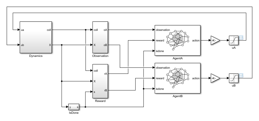

There are two variants of the predefined Simulink pusher environment, which differ by the agent action space.

• Discrete — The agent can apply a force which is quantized along the horizontal and vertical dimensions in five points consisting of -MaxForce, -MaxForce/2, 0, MaxForce/2, and MaxForce.

• Continuous — The agent can apply any torque within the range [-MaxForce,MaxForce].

Here, MaxForce is an environment property that you can change by accessing the workspace of the rlPusherModel model. For more information on other variables that you can change, see Dynamics. For more information on Simulink model workspaces, see Model Workspaces (Simulink) and Change Model Workspace Data (Simulink).

To create a predefined Simulink pusher environment, use rlPredefinedEnv as follows, depending on the desired action space:

• Discrete action space

  env = rlPredefinedEnv("PusherModel-Discrete")

  env = 
  
  SimulinkEnvWithAgent with properties:
  
             Model : rlPusherModel
        AgentBlock : [
                       rlPusherModel/AgentA
                       rlPusherModel/AgentB
                     ]
          ResetFcn : []
    UseFastRestart : on

• Continuous action space

  env = rlPredefinedEnv("PusherModel-Continuous")

  env = 
  
  SimulinkEnvWithAgent with properties:
  
             Model : rlPusherModel
        AgentBlock : [
                       rlPusherModel/AgentA
                       rlPusherModel/AgentB
                     ]
          ResetFcn : []
    UseFastRestart : on

Note

When training or simulating an agent within a Simulink environment, to ensure that the RL Agent block executes at the desired sample time, set the SampleTime property of the agent object appropriately.

For more information on Simulink environments, see SimulinkEnvWithAgent and Create Custom Simulink Environments.

Environment Visualization

Unlike the MATLAB pusher environment, for the Simulink pusher environment you do not have access to a plot function. However, the same plot described in the Environment Visualization section of the MATLAB Pusher Environment, is displayed automatically by the Simulink model when it is executed by the simulation or training function.

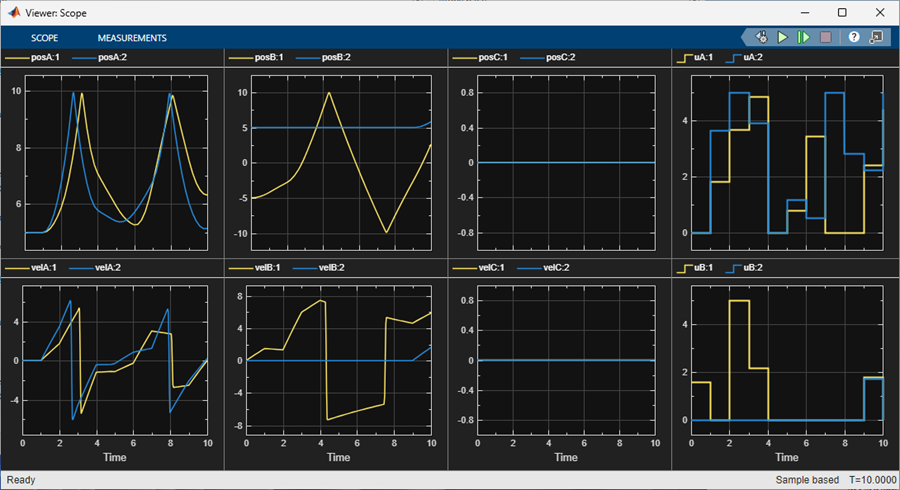
An additional visualization, from a Simulink Floating Scope and Scope Viewer (Simulink) block, automatically displays when the model is executed. This visualization shows how the positions and velocities of the three disks, and the forces applied by the agents, evolve during the current episode.

Environment Properties

The environment properties that you can access using dot notation are described in SimulinkEnvWithAgent.

Dynamics

The continuous-time environment dynamics are described in the Pusher Environment Dynamics section of MATLAB Pusher Environment. During simulation, the Simulink solver integrates the dynamics according to the selected solver, while the RL Agent block executes at discrete intervals according to the sample time specified in the SampleTime property of the agent.

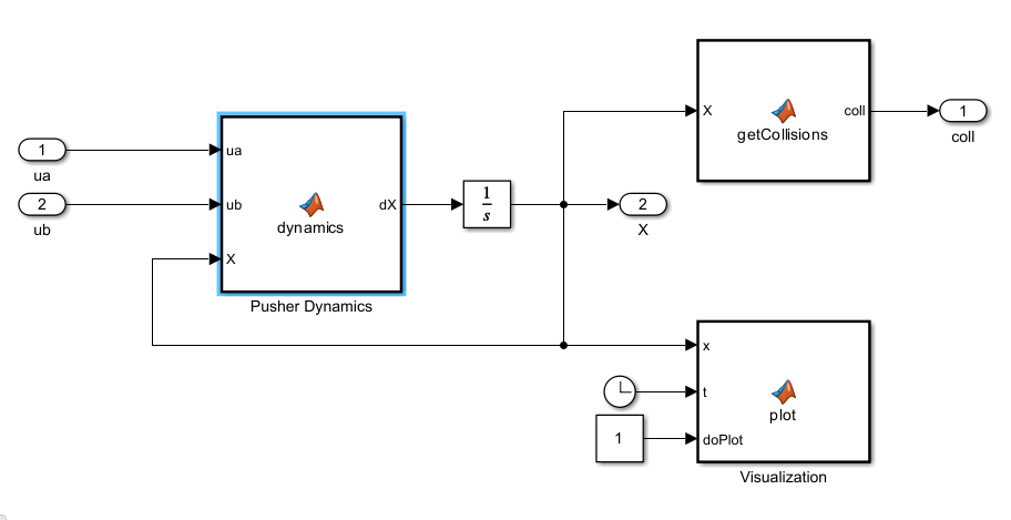
The Dynamics subsystem of the rlPusherModel model relies on three MATLAB Function (Simulink) blocks to call the same code used for the MATLAB Pusher Environment environment to calculate the dynamics and the collision flags and to visualize the disks on the plane.

The parameters that define the system dynamics are stored in the model workspace.

Variable	Description	Default
ContactStiffnessCoefficient	Coefficient for computing contact forces (contact forces are modeled as static spring forces). For more information, see Dynamics.	1000
Height	Height in meters of the rectangular region in which disks move. Disks bounce off the boundary of this region when attempting to move through it.	20
MaxForce	Maximum force in newtons that an agent can apply to its disk	5
ParticleMass	Masses of the disks in kilograms, specified as [mA,mB,mC], and mA and mB are the masses of the disks guided by agents A and B, respectively, and mC is the mass of the third disk.	[1 1 10]
ParticleRadius	Radii of the disks in meters, specified as [rA,rB,rC] where rA and rB are the radii of the disks guided by agents A and B, respectively, and rC is the radii of the third disk.	[0.25 0.25 0.75]
TaskRadius	Radius of the circular boundary in meters	8
VelocityDampingCoefficient	Damping on disks motion (viscous friction) in newtons per second over meters, specified as [dA,dB,dc], where dC and dB are the damping coefficients for the masses guided by agents A and B, respectively, and dC is the damping coefficient for the disk that the agents have to move out of the task circle.	[0.1 0.1 10]
Width	Width in meters of the rectangular region in which disks must stay. Disks bounce off the boundary of this region when attempting to move through it.	20
X0	Initial value of the environment state (positions and velocities of the three disks)	[5 5 -5 5 0 0 0 0 0 0 0 0]'

For more information on Simulink model workspaces, see Model Workspaces (Simulink) and Change Model Workspace Data (Simulink).

Actions

Like the predefined MATLAB pusher environment, each agent uses its own action channel, which carries a two-element vector containing the (normalized) forces applied by the agent to its disk in the x (positive-right) and y (positive-up) directions.

For the detailed description of the action spaces for the discrete and continuous versions of this environment, see the Actions section of MATLAB Pusher Environment.

Unlike the MATLAB pusher environment, the action space of the agent is fixed. Both agents either have a discrete action space in the discrete environment or they have a continuous action space in the continuous environment. You cannot set the type of an agent action space after you create the environment.

Observations

As for the predefined MATLAB pusher environment, each agent has its own single observation channel, which carries a nine-element vector containing the position and velocity of its disk, the position and velocity of disk C, and a flag indicating whether a collision with disk C is occurring.

In this environment, the observation signal for each agent is calculated within the Observation subsystem of the rlPusherModel model.

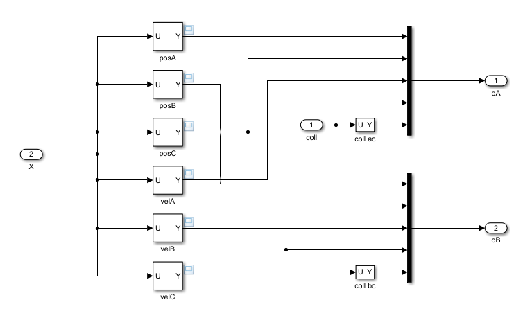
For the detailed description of the agents observation spaces, see the Observations section of MATLAB Pusher Environment.

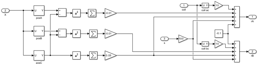
Reward

The reward signal for each agent is described in the Rewards section of MATLAB Pusher Environment.

In this environment, the reward signal for each agent is calculated within the Reward subsystem of the rlPusherModel model.

Reset Function

The environment has no default reset function. However, you can set your own reset function to set the initial state of the system every time a simulation is started to train or simulate the agents.

For example, set the initial state so that the agent disks stand still near the upper corners of the default allowed rectangle.

env.ResetFcn = @(in)setVariable(in,...
          "X0",[7 7 -7 7 zeros(1,8)]', ...
          "Workspace","rlPusherModel");

Here, you use setVariable (Simulink) to set the variable X0 to [7 7 -7 7 zeros(1,8)]' in the Simulink.SimulationInput (Simulink) object in. The value of X0 that you specify overrides the existing X0 value in the model workspace for the duration of the simulation or training. The value of X0 then automatically reverts to its original value when the simulation or training completes.

Create Default Agents for this Environment

The environment observation and action specifications allow you to create an agent that works with your environment. For example, for the version of this environment in which both agents have a continuous action space, create default PPO and SAC agents.

agentA = rlPPOAgent(obsInfo{1},actInfo{1})
agentB = rlSACAgent(obsInfo{2},actInfo{2})

agentA = 

  rlPPOAgent with properties:

            AgentOptions: [1×1 rl.option.rlPPOAgentOptions]
    UseExplorationPolicy: 1
         ObservationInfo: [1×1 rl.util.rlNumericSpec]
              ActionInfo: [1×1 rl.util.rlFiniteSetSpec]
              SampleTime: 1


agentB = 

  rlSACAgent with properties:

        ExperienceBuffer: [1×1 rl.replay.rlReplayMemory]
            AgentOptions: [1×1 rl.option.rlSACAgentOptions]
    UseExplorationPolicy: 1
         ObservationInfo: [1×1 rl.util.rlNumericSpec]
              ActionInfo: [1×1 rl.util.rlFiniteSetSpec]
              SampleTime: 1

Set the agents sample time so that the RL Agent blocks execute at the desired rate.

agentA.SampleTime = 0.05;
agentB.SampleTime = 0.05;

If needed, modify the agent options using dot notation.

agentA.AgentOptions.CriticOptimizerOptions(1).LearnRate = 1e-3;
agentA.AgentOptions.CriticOptimizerOptions(2).LearnRate = 1e-3;
agentA.AgentOptions.ActorOptimizerOptions.LearnRate = 1e-3;
agentA.AgentOptions.CriticOptimizerOptions(1).LearnRate = 1e-3;
agentB.AgentOptions.CriticOptimizerOptions(2).LearnRate = 1e-3;
agentB.AgentOptions.ActorOptimizerOptions.LearnRate = 1e-3;

You can now use both the environment and the agent as arguments for the built-in functions train and sim, which train or simulate the agent within the environment, respectively.

You can also create and train agents for this environment interactively using the Reinforcement Learning Designer app. For an example, see Design and Train Agent Using Reinforcement Learning Designer.

For more information on creating agents, see Reinforcement Learning Agents.

Step Function

Because this is a Simulink environment, calling the step function is not supported. For an example on how to build a custom training loop using a Simulink environment, see Custom Training Loop with Simulink Action Noise.