RF Data Analysis and System Design for Scientific Applications, Part 3: Simulating RF-Controlled Components at the System Level
From the series: RF Data Analysis and System Design for Scientific Applications
Integrate RF chains together with digital signal processing algorithms and control logic in feedback and feedforward configurations. Explore different architectural choices and develop algorithms to correct and calibrate RF impairments at the system level.
Published: 19 Jun 2023
So which type of components can you specify in circuit envelope and you can simulate? So I'm going to go through the different components and why you might want to use that. Yes, so you have different categories of components. You have a linear element-- or elements that you can specify in the frequency domain-- such as S-parameters, transmission lines, lamp component, RLCs, filters, alternators, couplers, circulator, dividers, phase shifters, antennas, elements. These are all linear, linear time invariant.
We have nonlinear components-- amplifiers, power amplifiers, mixer, as well as system blocks, entire subsystems, like modulator, demodulator with IQ components, including channel select and image reject filters, for example. And then you have basic components, for example, to generate noise if you want to inject noise in specific parts of your system.
By the way, each of the nonlinear components allow you to specify noise, both noise as specified in terms of noise figure or, for example, in terms of noise parameters, including the impedance relationship or, for example, using color noise, so if you have a spectral distribution for your noise.
And then you have some of the components that I find more interesting and that refer to what Belid was asking. You can have variable components such as VGAs, attenuator, phase shifters, RLC. So these are components with behavior changes in the time domain. And we will see them in a second.
For the linear component S-parameters, we go back-- S-parameters, essentially, is the-- I'm going to say the overarching category of a component that is linear and frequency dependent. For simulating them in the time domain, by default, we use the rational fitting. We already talked about rational fitting.
We automatically create an equivalent Laplace transfer function representing the S-parameters of the object. And we use that pole-zero representation for simulating the network in the time domain. For the hardcore engineers that want to use inverse FFT, we also provide a convolution-based approach. We provide both approaches. Sometimes there are reasons why you might still want to use inverse FFT.
You might wonder why. I'll give you a very simple example because it's probably one of my favorite ones. Let's say that you have a component where you specify only the magnitude of the S-parameters, but you don't know anything about the phase. Let's say that you have a perfect filter with a certain mask. You know what is the filter specification in the frequency domain, but you don't know exactly what the phase is going to be.
Now, if you want to fit that component using rational fitting, rational fitting will not manage. Why? Because it needs the phase information to create the causal component. So for those type of components-- for example, you're using a convolution-based approach or an inverse FFT, essentially, or a frequency domain approach is best. Essentially, what happens, it takes the amplitude to create an equivalent FIR filter for the simulation of your components. And you have a lot of other components that are given in terms of specification, so the role-behavioral models that you can use in your simulation.
For non-linear components, there is a lot to say here. So you can provide the specifications in terms of IP2, IP3 saturation, 1 dB compression point. You can also provide AM-AM and AM-PM characteristics. So if you have a lookup table representing the linearity of your component, you can use those.
If you have a mixer within the modulation tables, you can directly import into inter-modulation tables in your simulation. So this is important if your mixer has and you want to model disperse effect on your system. And yeah. And also, if you're working on the power amplifiers, power amplifiers, they often-- say, gallium nitride or some of the more exotic 3G semiconductor technology-- those tend to exhibit memory-dependent effects, which I can tell you are really hard to model.
So you can be in a situation where not only your component is nonlinear, but the nonlinearity depends on the previous state of your input signal. Now, if your input signal is a sinusoid, it's relatively simple. If your input signal is modulated, then memory will have a large impact. So the output signal not only will depend on the instantaneous input but also on previous states of the input signal.
So for these type of systems, we do provide a generalized memory polynomial approach where you can describe both the effects on nonlinearity and memory effects. It's like combining nonlinearity with S-parameters, if you like, a way to think about it. Noise, we talked about it. A lot of the components, most of the components include the noise generation for active components, such as amplifiers, mixer. You can specify, for example, the noise figure or the spot noise data.
For passive components, such as S-parameters, by default, if the S-parameters are passive, then noise is generated that is proportional to the attenuation that the block introduces so you can automatically get the noise that, for example, an attenuator introduces. So let's say an attenuator gives an attenuation of 3 dB, then it will have automatically a noise figure of 3 dB. And you can also have noise sources that you can inject on your circuit. And you can also model phase noise on your local oscillators.
Last but not least, my favorite blocks, honestly, tunable blocks. They are blocks such as-- for example, these variable alternator, let's say, or this variable capacitor, where the attenuation that the block provides depends on the instantaneous value of its input signal. So in this case, you see that each of these blocks have a physical port. This is like you see a node on an electrical network so you can connect this to another inductor capacitor and the Kirchhoff laws will be solved for this terminal.
But it also has a control port, and the control port represents the actual value that this inductor offers to the network. And it can change at every time step of your simulation. This is very interesting because now we have components such as a capacitor, inductor, or the switch that are steady state, are linear. But as soon as we apply a control signal that changes the characteristic of the system, they actually become nonlinear. So a time-varying capacitor is effectively a nonlinear component. A time-variant switch is effectively a nonlinear component.
What you can do with this is now you can start inserting your RF network into a larger system and, for example, make it dependent on the signals themselves, on the operating conditions themselves. So in this case, for example, we have a variable gain amplifier, where we have the gain that depends on the output power. So here, the output of this variable gain amplifier will measure the power. Depending on the power, we change the gain of our VGA.
Think about it if you want to do, for example-- to model a feedback loop, that if your power goes to up, you want to switch off your VGA, for example, just to make an example. To avoid it, it breaks down. Or think about it when you want to have, for example, to build a system that compensates for temperature deviation. So you know that when your variable gain amplifier heats up, because it dissipates a lot of power, then the gain might go down or might go up.
With this type of feedback, you can actually model this type of effect. And actually, block goes beyond that. Because not only the gain changes instantaneously depending on the feedback or the output power, but also, its nonlinear characteristics, such as the IP2 or the IP3, change as a function of the gain, so not only the gain that is the desired effect but [AUDIO OUT] of the system.
A few more blocks, we have testbenches, very useful to verify that your chain is behaving like you are expecting. So let's say that I have a chain, I have a system I want to measure what is the noise figure, the IP3, what is the gain, what are the S-parameters. You have testbenches that allow you to apply a stimulus and look at the output to verify that your network is what it is or is modeling what it's supposed to model.
And last but not least, if your system is not behaving, if you don't find the component that you're looking for, you can actually create your own component. So we do actually provide a language that allows you to describe the network equations, physical network equations in terms of voltages and currents, to represent any arbitrary component to extend the library.
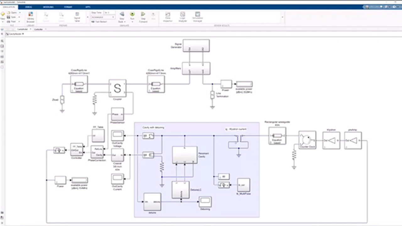
So with this, let's go back to our model where we started at the beginning and see how we use the RF Blockset and the circuit envelope to model this linear particle accelerator. So just bear with me for a second. I'm going to do a little bit, again, of cleanup. I'm going to close my model. How it integrates RF Blockset and the circuit envelope simulation within Simulink and within a platform where we can model and simulate control systems.
So what do we have here? So we have a signal generation this generates. It's just a fixed signal, essentially, with a fixed phase or with a phase that is as constant as possible. This is fed through a series of lines and couplers. And the phase of the signal gets probed at different section. This is just one part of the section. And the signal is amplified to a certain power level.
In this case, we actually had two phase lines, a long one and a short one. But we are only using the phase of one of the two lines. We plot the phase of the signal, and we use this phase to control the phase of our resonant cavity. So in this case, essentially, we use the reference and we compute the difference between the phase of the signal, or the output of the cavity, and our reference phase to control the control algorithms so that it adjust the de-excitation, essentially, through the cavity.
Next to this, we also have a resonant cavity that is resonant as a function of the signal that gets applied to that. But we also have a detuning mechanism due to the Lorentz force. So in other words, the cavity gets disturbed, and the frequency and the phase at which it resonates varies over time due to this detuning effect.
When we look at this model overall, you notice-- if you have, at least, good eyes-- two things at the first level-- one, that they have two different types of signals. So you see we have certain lines that are dark blue, like these ones, and certain lines that are black and marked with a single, unidirectional arrow.
Here, we are really combining two domains of simulations. The signals that are indicated with a black arrow, essentially, they are Simulink signals. They don't have really any physical meaning. They are a signal. They could represent a voltage. They could represent a current. They could represent a temperature. They could represent a force. They could represent anything. It is up to you as a user to define what is the meaning of that specific signal.
And the blocks are all unidirectional. So in a way, they behave just like a function. You get a sample in, you get a sample out. They can have internal states, but there is not such a thing as the input depends on the output unless you have a feedback loop that is separately or explicitly modeled.
The signals that are indicated in blue, they represent an electrical connection. So effectively, these nodes are solved in the domain of Kirchhoff, in the domain of voltages and currents, which means that, for example, if I look at this rigid line, the signal will be propagating from the signal generation to the signal through the line itself through the coupler. If there is an impedance mismatch, part of the energy will reflect back and will affect the remaining part of the chain.
So this is the biggest thing that I want to highlight here, that we are really putting together a physical model representation of our entity, of our plant, together with a signal-level representation of our algorithms. So really, this puts together RF plus control algorithms, control logic, or any digital signal processing that you want to put in your system.
If you look at the signal generation, well, this is fairly straightforward. I just have a CW tone to which I can add some phase noise. Essentially, this is multiplied to the power of 2 because we have two frequencies, one that is the double of the other one. And then we feed this-- this is all in the Simulink domain. And you see here, we feed the Simulink domain into a port that converts the signal to an equivalent power centered around 352 megahertz.
So now with this input port, we convert from the signal domain to the physical domain. To the left is unidirectional. To the right is bidirectional. And effectively, we are in the domain of the RF signals.
Now we can follow our signal through our chain. We have a couple of amplifiers, in this case, circulators as well to guarantee isolation. So if there is energy that is reflected back, it will be dissipated on this resistor, just to make an example. We follow it through a transmission line that is equation based, where we have a certain length, certain loss, repeater meters. So we have a physical model.
We could have S-parameters here, just like we've seen before. Or we could have-- in this case, this is all big RF components. These are big pieces of metal. Those are big waveguides. But if you work with lower power, it could be a PCV. It could be a transmission line, a coaxial or whatever.
We have a coupler. This, again, is a behavioral model of a coupler but which is actually represented by its-- it's not a behavioral model, but it's actually represented by its S-parameters again. So we can look at different level of isolation and the coupling factors. At the couple port, now we probed our output signal, and we actually probe the phase of our signal.
So you see here, we extracted the phase of our reference line. We also have a manual switch that during the simulation, we can say I want the actual phase of the reference line, or maybe I want to experiment with a fixed phase just to verify that the behavior of my feedback loop is what I'm expecting. And then we apply the reference line through and compare it with the phase of the output voltage of our cavity.
So you can see here, essentially, we compute the difference between the two. And we use this to control as an input as, essentially, the error that we make between the reference phase line and the output cavity. And we use this error to control our correction algorithm or our control algorithm.
So under this last block here, what you find here is actually the actual controller, essentially is a PID controller that allows you to adjust the excitation to your cavity so that it keeps the phase aligned with our reference line. So again, this is the excitation that gets converted.
You see another input port where we can go from the control domain, from the signal domain, into, essentially, an ideal current that gets injected to a chain of amplifier with the transformer that gets applied to our resonant cavity. Now, if you look at the cavity, a good way to represent the cavity resonance structure is by having an inductor in the capacitor. That's, I would say, electronics 101.
Again, what you find here is two variable components, variable inductor and the variable capacitor. And the value of the inductors and the capacitance is not constant but, as you can see, changes throughout the simulation. So these values actually LLC, are a function of a detuned algorithm.
This is also quite interesting because now to model the detune, I actually have a MATLAB function. So you see how you can really integrate your own algorithms within a simulation platform. So in this case, you see it's fairly straightforward. The mathematics is not really rocket science.
But essentially, you have the value of C and L that depends on the detuned value of this delta and the detuned value-- I'm going to go up in the hierarchy-- actually depends on the voltage at the terminal of our cavity. That's essentially how we are closing the loop. Overall, what we have-- well, you will see that we have a lot of simulation value.
But essentially, we have a reference line that controls the phase of our cavity. And they say this is our control loop and the detuned loop that is inside the simulation. So we have a feedback loop inside the feedback loop. This is, really, a situation that is really hard to predict what's going to happen.
We just pen and paper in the sense that when you do this with pen and paper, you have to have a certain assumption, like the system behaves linearly, for example. It's really hard to predict what happens if I suddenly start injecting process to my cavity or if there is a disturbance or if there is a nonlinearity, for example, coming in from the just to make an example.
So you start with a linear analysis. But as you evolve your model, you check it with your linear analysis. You check the different assumptions that you're making. But you use the model as essentially as a digital twin, if you like-- if you want to use this word-- of your actual system.
And as you run the simulation, actually, you see that it's fairly fast. And again, we can look at the different-- actually, this model, I think that it has a couple of millions of scopes, essentially, spread all over the model to allow you to check at every stage what's happening. I'm opening up them, but they are actually coming up on the other screen. So just bear with me as I drag a few of them here.
And then I'm just dragging them from one screen to the next just to give you an idea of the type of results that you can get and the type of insights that you can get throughout your simulation. Good. So let me put this one down. So we have, like I was saying before, quite a few scopes.
So you see, this is the phase difference between the reference line and the output of the cavity. This is our error signal. This is the control signal. This is the error signal. You see the timing response of the cavity in terms of voltage and current. Of course, they are related, so this is not surprising. But you also see, for example, the effects of the tuning and so how the detunes place-- this is the detune offset, the delta that we saw before to control our values of resistor and capacitors.
Good. So what we've seen here, feedback loop on the control, modeling of the reference signal using the RF system, modeling of the amplifiers, like we described before with circuit envelope, and then monitor, monitor, monitor, checking every single node of the network.
So, to summarize, we saw quite a bit, actually, in the past hour and a little bit. We started with RF data analysis, then for linear components, then we went to budget analysis for nonlinear components, introduced harmonic balance and circuit envelope simulation, and then we closed the loop.
Featured Product
Simulink
Up Next:

Related Videos:


Seleccione un país/idioma
Seleccione un país/idioma para obtener contenido traducido, si está disponible, y ver eventos y ofertas de productos y servicios locales. Según su ubicación geográfica, recomendamos que seleccione: United States.
También puede seleccionar uno de estos países/idiomas:
América
- América Latina (Español)
- Canada (English)
- United States (English)
Europa
- Belgium (English)
- Denmark (English)
- Deutschland (Deutsch)
- España (Español)
- Finland (English)
- France (Français)
- Ireland (English)
- Italia (Italiano)
- Luxembourg (English)
- Netherlands (English)
- Norway (English)
- Österreich (Deutsch)
- Portugal (English)
- Sweden (English)
- Switzerland
- United Kingdom (English)