FMCW Radar for Autonomous Vehicles | Understanding Radar Principles
From the series: Understanding Radar Principles
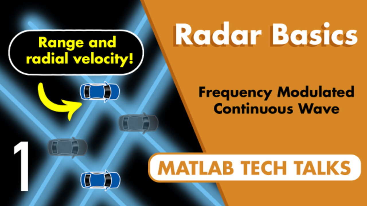
Watch an introduction to FMCW radar and why it’s a good solution for autonomous vehicle applications. This demonstration will show how FMCW radar can measure range and radial velocity for multiple targets at once using the Doppler effect, beat frequency, and frequency modulation.
Published: 13 Jun 2022
Radar is an important part of autonomous vehicles because it allows the vehicle to detect objects and estimate their parameters from a distance, which it can then use to make decisions. And applications for automotive vehicles range from blind spot detection and rear collision warning and adaptive cruise control up to tracking and classifying objects like pedestrians and cyclists and other vehicles.
And for flying vehicles, radar is used for object affordance and for measuring altitude. And there are a host of other uses for commercial vehicle applications. But in order for radar to be a practical solution for these applications it needs to be relatively low-power, small form factor, and low cost.
And part of how that is accomplished-- but certainly not the complete story-- is with frequency modulated continuous wave radar, or FMCW. And so what I want to do in this video is talk just a little bit about why FMCW is a good solution for autonomous vehicle applications. But, mostly, I want to try to build up a little intuition around how FMCW radar can measure range and radial velocity for multiple targets all at once. I hope you stick around for it. I'm Brian, and welcome to a MATLAB Tech Talk.
To begin, let's just look at the second half of FMCW. What is continuous wave radar? And as the name suggests, this is a type of radar system that transmits a known stable frequency continuously. That wave propagates out, reflects off an object, and is received continuously by the radar.
Now, this is in contrast to pulsed radar, where short-duration but high-energy pulses are emitted in series. With pulsed radar, in its simplest form, determining range and radial velocity is relatively intuitive. I mean, we can determine the distance to an object by timing how long it takes the pulse to travel the round trip, and then multiply it by the speed of light to get the distance, and then divide by two to get the one-way distance. And we can measure radial velocity simply by looking at the change in distance between two successive pulses.
Now, there are other more complex and more accurate ways to determine these measurements with pulsed radar. But I just wanted you to see that there is a simple and easy to understand solution. On the other hand, getting these measurements isn't necessarily obvious with continuous wave radar, since there is no start and end to a continuous signal that we can use to time how long it takes for the signal to travel the round-trip distance.
So why are we complicating matters by using continuous wave radar? Well, it comes down to size, weight, and power of the electronics and the specific applications of where we're going to use this radar. For example, in pulsed radar, the pulses need to be relatively powerful so that the return signal has enough energy to be detected over the short duration, often just a microsecond or so. And handling these large peak power loads can make the electronics larger and more expensive than continuous lower power loads.
And another reason is that pulsed radars have a minimum range that can be detected of about half the length of the pulse. And this is because the trailing edge of the pulse must be emitted before the leading edge returns. And as an example, the minimum detectable range is about 150 meters for a 1-microsecond pulse. And since autonomous vehicles usually need to measure objects within a few meters and have cheaper and smaller electronics, then continuous wave tends to be the best choice.
Now, getting range and radial velocity from continuous waves might not seem obvious at first. But this is where the Doppler effect, beat frequency, and frequency modulation come into play. Let's start with the Doppler effect. Imagine a radar sends out a signal at a fixed frequency. And if the radar and the object it's detecting are both stationary, then the signal will reflect off that object and come back to the radar at the same frequency, like bouncing off a mirror.
So here are the black transmit frequency is the exact same as the blue reflected frequency. However, if the object is moving towards the radar, then the reflected frequency is higher than the transmit frequency due to the fact that the later parts of the signal don't have to travel as far before being reflected. For example, this peak reflects off the object here. But the second peak only had to travel to this spot before being reflected, since the object moved closer. Therefore, it's caught up a little bit to the earlier peak of the signal that had to travel further. This increases the frequency proportional to how fast the object is moving.
And the opposite is true if the object is moving away. Then the reflected frequency is lower. In this way, the change in the frequency of the received signal can provide an estimate of the radial velocity of the object and its direction.
So the question now is, how can we detect these frequency changes? And the way that I have it drawn here, where the reflected signal is, like, half the frequency of the transmitted signal, then there is a really obvious difference between the two. However, something to note is that continuous wave radar is often in the microwave range of the spectrum, which means transmit frequencies that are tens of gigahertz. And for an object moving at a couple hundred of kilometers per second and slower, then the reflected frequency is only shifted by tens of kilohertz.
And so the frequency is only being shifted by 1/100,000%, not half or double like I've shown here. The two signals would be indistinguishable from one another on this screen if I drew them correctly. But detecting really tiny frequency differences is made much easier by looking at beat frequencies. And to show you how it works, I made this simple MATLAB app.
The transmit frequency from the radar, I'm setting to 100 gigahertz. The received signal comes back at a different frequency, which I can adjust with this slider. So here I'm going to just set it to 108 gigahertz, which means that the object is moving towards the radar.
And, again, this Doppler shift is much larger than anything an autonomous vehicle will see. But I want it to be able to show the beat frequency easily on this screen. All right. So at the radar, we have a known 100-gigahertz transmit signal. And we can compare it to the 108-gigahertz received signal.
And notice, initially, these two peaks line up with each other. And then, as time progresses, the faster frequency starts to lead the lower one. And, eventually, the peaks are exactly out of phase.
And if we keep going again the peaks line up, and then are out of phase, and then they line up again, and so on. This is the beat frequency. And to find this frequency, we can mix these two signals together by multiplying them. And we get this resulting waveform.
And, by the way, multiplying two sinusoids produces a signal that is composed of two new sinusoids, which we can see clearly in this waveform. There's this high-frequency component which comes from adding the transmit and received frequencies together, and then this low-frequency component that comes from subtracting the transmit and received frequencies. And this subtraction produces the beat frequency, which you can see lines up with the in-phase and out-of-phase portions of our two signals.
And when we're talking about two signals in the gigahertz, adding the transmit and received frequencies together produces something that is extremely fast. However, subtracting the two produces just the shift to Doppler, which, in this example, is 8 gigahertz. But remember, for practical applications, it would only be in the kilohertz range.
So we have a gigahertz signal superimposed with a kilohertz signal. And we could easily separate out the beat frequency with a low-pass filter. And as I increase the received signal frequency, you can see that the beat frequency increases as well. And, therefore, by looking at the much slower beat frequency, we can determine the radial velocity of the object.
However, there is a small problem with how I've set this up. If I toggle back and forth between 120 gigahertz and 80 gigahertz, you'll notice that the beat frequency doesn't change. The difference is 20 gigahertz regardless.
This is a radar system with just a real stage, a single transmit signal. And with this setup, we can determine the speed of the object but not the direction. We can't tell if it's coming towards the radar or moving away.
But this is where radar systems with complex stages come into play. Imagine that the radar sends out two orthogonal signals that are separated by 90 degrees of phase, so-called IQ signals. The IQ comes from the fact that the real component is called in-phase and the imaginary component is called quadrature.
But by generating these complex signals, we can now determine the direction of the object. When we mix the transmit and received signals, we get another complex signal where both the in-phase and quadrature components oscillate at the beat frequency. But in addition to that, notice that when I toggle between 80 gigahertz and 120 gigahertz, the in-phase component doesn't change, just like we saw before. But the quadrature component does move. And, therefore, by checking which of the signals is leading in phase, we can determine direction.
So, as a quick recap, we transmit IQ signals. They get Doppler shifted. And then, the received signals are mixed with the transmit signals to produce a beat frequency. And the beat frequency is proportional to radial velocity of the object. And its direction is given by which signal is leading in phase.
And that's pretty awesome on its own that we can get velocity from a continuous signal. But with autonomous vehicles, we want to measure range as well as velocity. And to do that, we need frequency modulation.
Distance doesn't cause a Doppler shift like velocity does. Instead, it produces a time shift because of the time it takes for the signal to travel to the object and back. The further the object, the more time it takes.
And with a fixed frequency signal, we can't detect this delay, since, again, there isn't a pulse or any other defining characteristic we can use to measure time. A delay of one period looks the same as two periods and the same as three, and, well, you get the idea.
We can see this more cleanly if we plot the frequency of the transmit signal as a function of time. With a fixed frequency, this is just a horizontal line. The Doppler shift lowers the frequency of the received signal if the object is moving away from the radar and raises the frequency if it's moving towards the radar. And we already know we can detect this beat frequency and direction by mixing the two IQ signals.
But for a stationary object at a distance, the received signal is just shifted horizontally. And, therefore, there is no beat frequency between the transmit and received signals. So to get around this problem, we can modulate the frequency.
For example, with linear frequency modulation, we essentially ramp the transmit frequency from some value, like 77 gigahertz, up to another one, like 81 gigahertz. And we do this over and over again, creating a sawtooth modulation pattern. Now, when the received signal is delayed in time, we do get two different frequencies at any given moment, and hence, a beat that can be measured. So we are able to determine range in a very similar way as we do velocity by mixing the transmit and received signals and measuring the beat frequency.
Unfortunately, with this setup, we have a slight problem that we need to address. The problem is we can't determine whether this beat frequency is caused by a time shift, like we see here, or by a Doppler shift, like this. And, worse than that, we can't tell if there's a combination of Doppler and a time shift. So we have two unknowns-- Doppler and time delay-- in just this single beat frequency.
Another way to visualize this is on a range Doppler chart. Again, for a single beat frequency, the object could have zero range and some Doppler, zero Doppler and some range, or a combination of the two. So the actual parameters of the object fall somewhere on this line. And in order to resolve these two unknowns, we essentially need a second beat frequency.
And there are many ways to accomplish this. For one, instead of a sawtooth modulation, we could use triangular modulation, where the frequency increases linearly and then decreases linearly. Now, when an object is moving away from the radar at zero range, the received frequency is lower, and we get two beat frequencies, one on the rising side of the triangle, which looks like a positive time delay, but then one on the falling side that looks like a negative time delay. In this way, the two time delays cancel out. And we can determine that range is zero, and therefore, the beat frequency is produced only by Doppler.
And when an object is at a distance but not moving, then both the rising and falling sides are delayed in time. And this, again, produces two different beat frequencies, one that looks like a positive Doppler and one that looks like a negative Doppler. Again, those cancel out, and we can determine that the object is not moving. Plus, by looking at these two beat frequencies, we can separate Doppler from range with any combination of the two.
Back on the range Doppler chart, the beat frequency for downward-sloping modulation produces a second possible set of answers. And the intersection of the two is the true range and Doppler of the object. Of course, these aren't crisp lines because of the range resolution of the radar, and there's noise and interference. But, conceptually, this is how triangular frequency modulation can determine range and radial velocity of a single object.
But, again, we have a problem here because autonomous vehicles often encounter many objects. And sometimes, there is more than just one in the line of sight of the radar beam. For example, if there are two objects in the radar beam, then each object will produce its own reflection, which means that there are two different beat frequencies for the rising slope and two for the falling slope. So, in total, we have four different beat frequencies that we need to interpret.
If we go back to the range and velocity plot, this is equivalent to two Xs, centered over the real range and velocity of the two objects, one line for each beat frequency. Unfortunately, when we do this, we're actually left with four intersections, or four potential objects, and no clear way to distinguish which are the two real ones and which are two ghost objects.
All right. So now we need to get around this problem. And there are several clever things that we could do. For one, we could change the triangular modulation such that it alternates between two triangles of different slopes.
With this setup, a Doppler shift would be the same for all four slopes. But if you apply a range shift, the apparent delay associated with the steeper slope is less than the other one. And this provides us with additional equations, or additional beat frequencies that we can use to solve for the additional unknowns that come from ghost detections.
Practically speaking, essentially, all we're doing with the second triangle is adding two more Xs on our range Doppler chart at different slopes. And with this additional information, we can determine where the real objects are versus the ghost objects, as long as they're separated enough that they're outside of all of the fuzz created by noise interference and all of that.
And so with this multiple triangle approach, you need N unique triangles for N number of objects in the field of view. So if there's five objects, then you need five different sloped triangles, which can start to get pretty cluttered.
But, luckily, this isn't the only way to resolve multiple objects in the field of view. We can modulate the frequency of the continuous wave signal in other ways that can actually more easily separate speed and distance for many targets at once. And I'm not going to go into them here, but I've left some really good resources and MATLAB examples that show you how to set up and interpret other modulation schemes, like multiple frequency shift keying, or MFSK, and fast chirp.
And the idea behind all of them is that through clever frequency modulation of a continuous wave, we can look at the beat frequency that is generated when we mix the transmit and received signals together to determine range and radial velocity of multiple targets in the field of view.
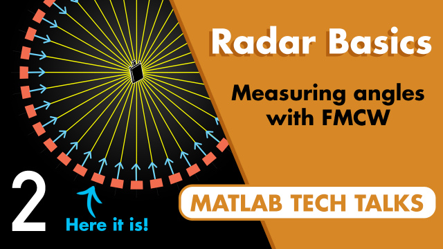
All right. So that's where I'm going to leave this for now. In this video, we talked about measuring range and velocity of objects. However, for autonomous vehicle applications, we usually want to know more than just that. We also want to know the object's azimuth and elevation relative to the radar to get a sense of where it is in 3D space and to have an understanding of its size and shape. And that's what we're going to talk about in the next video.
So if you don't want to miss that or any other future Tech Talk videos, don't forget to subscribe to this channel. And if you want to check out my channel, Control System Lectures, I cover more control theory topics there as well. Thanks for watching, and I'll see you next time.


Seleccione un país/idioma
Seleccione un país/idioma para obtener contenido traducido, si está disponible, y ver eventos y ofertas de productos y servicios locales. Según su ubicación geográfica, recomendamos que seleccione: United States.
También puede seleccionar uno de estos países/idiomas:
América
- América Latina (Español)
- Canada (English)
- United States (English)
Europa
- Belgium (English)
- Denmark (English)
- Deutschland (Deutsch)
- España (Español)
- Finland (English)
- France (Français)
- Ireland (English)
- Italia (Italiano)
- Luxembourg (English)
- Netherlands (English)
- Norway (English)
- Österreich (Deutsch)
- Portugal (English)
- Sweden (English)
- Switzerland
- United Kingdom (English)