edgeConstraints
Restricciones de borde en el gráfico de pose
Sintaxis
Descripción
measurements = edgeConstraints(poseGraph)
[ también devuelve las matrices de información para cada borde. La matriz de información es la inversa de la covarianza de la medida de pose.measurements,infoMats] = edgeConstraints(poseGraph)
[ devuelve restricciones de borde para los ID de borde especificados.measurements,infoMats] = edgeConstraints(poseGraph,edgeIDs)
Ejemplos
Este ejemplo muestra cómo identificar y eliminar cierres de bucles espurios del gráfico de pose. Para hacer esto, puede modificar la pose relativa de un borde de cierre de bucle e intentar optimizar el gráfico de pose con y sin eliminar el cierre de bucle espurio automático y comparar los resultados.
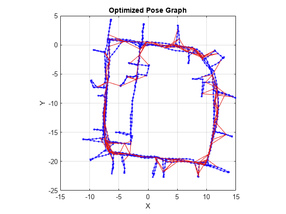
Cargue el Conjunto de datos de Intel Research Lab que contiene un gráfico de pose 2-D. Optimiza el gráfico de pose. Traza el gráfico de pose con las identificaciones desactivadas. Las líneas rojas indican cierres de bucle identificados en el conjunto de datos.
load intel-2d-posegraph.mat pg
optimizedPG = optimizePoseGraph(pg);
show(optimizedPG,IDs="off");
title("Optimized Pose Graph")
Modifique la postura relativa del borde de cierre del bucle 1386 a algunos valores aleatorios.
loopclosureId = 1386;
nodePair = edgeNodePairs(optimizedPG,loopclosureId);
[relPose,infoMat] = edgeConstraints(optimizedPG,loopclosureId);
relPose(2) = -5;
relPose(3) = 1.5;
addRelativePose(optimizedPG,relPose,infoMat,nodePair(1),nodePair(2));
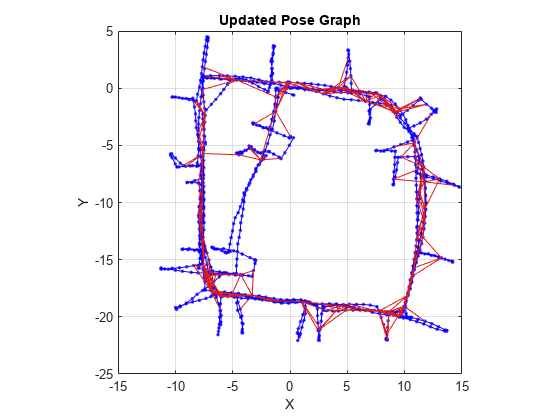
Optimice el gráfico de pose sin recortar el cierre automático del bucle. Trace el gráfico de pose optimizado para ver el ajuste deficiente de los nodos con cierres de bucle.
[updatedPG,solutionInfo] = optimizePoseGraph(optimizedPG);
show(updatedPG,IDs="off");
title("Updated Pose Graph")
Ciertos cierres de bucle deben recortarse del gráfico de pose. Utilice la función trimLoopClosures para recortar estos cierres de bucle defectuosos. Establezca el umbral de truncamiento y las iteraciones máximas para los parámetros del recortador.
trimParams = struct("TruncationThreshold",0.5,"MaxIterations",100);
Generar opciones de solver .
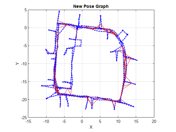
solverOptions = poseGraphSolverOptions("g2o-levenberg-marquardt");Utilice la función trimLoopClosures con los parámetros del recortador y las opciones del solucionador. Trace el nuevo gráfico de pose para ver que se eliminaron los cierres de bucle incorrectos.
[newPG,trimInfo] = trimLoopClosures(updatedPG,trimParams,solverOptions);
show(newPG,IDs="off");
title("New Pose Graph")
Argumentos de entrada
Argumentos de salida
Capacidades ampliadas
Historial de versiones
Introducido en R2019b