factorGraph
Marco basado en gráficos para la estimación del estado de múltiples sensores
Desde R2022a
Descripción
Un objeto factorGraph almacena un gráfico bipartito que consta de factores conectados a nodos variables. Los nodos representan las variables aleatorias desconocidas en un problema de estimación, como las poses de los robots, y los factores representan restricciones probabilísticas en esos nodos, derivadas de mediciones o conocimientos previos. Durante la optimización, el gráfico de factores utiliza todos los factores y los estados actuales de los nodos para actualizar los estados de los nodos.
Para obtener más información sobre el gráfico de factores y cómo usarlo, consulte Gráfico de factores para SLAM.
Creación
Sintaxis
Descripción
fg = factorGraphfactorGraph vacío.
Propiedades
Funciones del objeto
Ejemplos
Cree una matriz de posiciones de los puntos de referencia para usar en la localización y las poses reales del robot para comparar la estimación del gráfico de factores. Utilice la función auxiliar exampleHelperPlotGroundTruth para visualizar los puntos de referencia y la trayectoria real del robot.
gndtruth = [0 0 0;
            2 0 pi/2;
            2 2 pi;
            0 2 pi];
landmarks = [3 0; 0 3];
exampleHelperPlotGroundTruth(gndtruth,landmarks)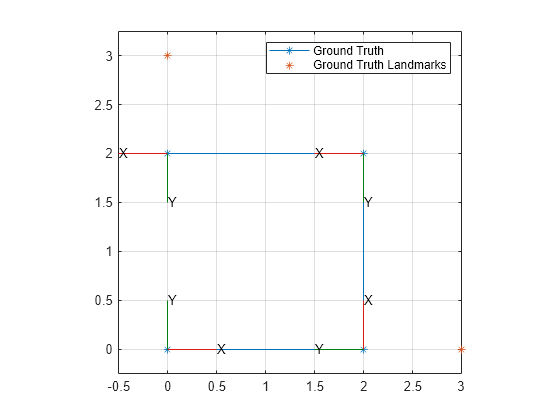
Utilice la función auxiliar exampleHelperSimpleFourPoseGraph para crear un gráfico de factores que contenga cuatro poses relacionadas por tres factores de dos poses en 2D. Para obtener más detalles, consulte la página del objeto factorTwoPoseSE2.
fg = exampleHelperSimpleFourPoseGraph(gndtruth);
Crear factores punto de referencia
Genere ID de nodo para crear dos ID de nodo para dos puntos de referencia. Los nodos de pose segunda y tercera observan el primer punto de referencia, por lo que deben conectarse a ese punto de referencia con un factor. Los nodos de pose tercero y cuarto observan el segundo punto de referencia.
lmIDs = generateNodeID(fg,2);
lmFIDs = [1 lmIDs(1);  % Pose Node 1 <-> Landmark 1
          2 lmIDs(1);  % Pose Node 2 <-> Landmark 1
          2 lmIDs(2);  % Pose Node 2 <-> Landmark 2
          3 lmIDs(2)]; % Pose Node 3 <-> Landmark 2
Defina las medidas de posición relativa entre la posición de las poses y sus puntos de referencia en el marco de referencia del nodo de pose. Luego agrega algo de ruido.
lmFMeasure = [0  -1; % Landmark 1 in pose node 1 reference frame
             -1   2; % Landmark 1 in pose node 2 reference frame
              2  -1; % Landmark 2 in pose node 2 reference frame
              0  -1]; % Landmark 2 in pose node 3 reference frame
lmFMeasure = lmFMeasure + 0.1*rand(4,2);
Cree los factores de referencia con esas medidas relativas y agréguelos al gráfico de factores.
lmFactor = factorPoseSE2AndPointXY(lmFIDs,Measurement=lmFMeasure);
addFactor(fg,lmFactor);
Establezca el estado inicial de los nodos de puntos de referencia en la posición real de los puntos de referencia con algo de ruido.
nodeState(fg,lmIDs,landmarks+0.1*rand(2));
Optimizar gráfico de factores
Optimice el gráfico de factores con las opciones de solver predeterminadas. La optimización actualiza los estados de todos los nodos en el gráfico de factores, por lo que se actualizan las posiciones del vehículo y los puntos de referencia.
rng default
optimize(fg)
ans = struct with fields:
InitialCost: 0.0538
FinalCost: 6.2053e-04
NumSuccessfulSteps: 4
NumUnsuccessfulSteps: 0
TotalTime: 4.9480e-04
TerminationType: 0
IsSolutionUsable: 1
OptimizedNodeIDs: [1 2 3 4 5]
FixedNodeIDs: 0
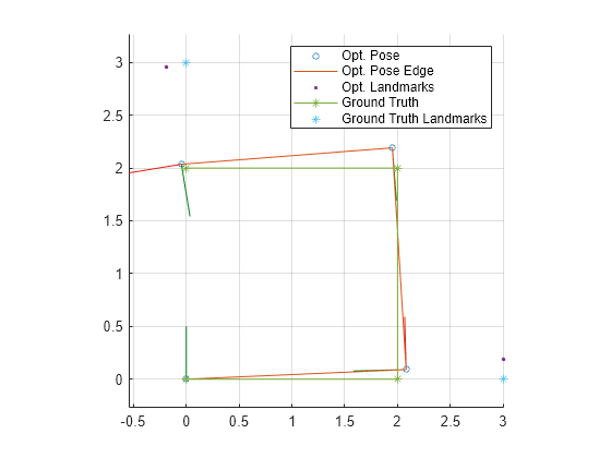
Visualice y compare resultados
Obtenga y almacene los estados de nodo actualizados para el robot y los puntos de referencia. Luego, trace los resultados, comparando la estimación del gráfico de factores de la trayectoria del robot con ground-truth del robot.
poseIDs = nodeIDs(fg,NodeType="POSE_SE2")poseIDs = 1×4
0 1 2 3
poseStatesOpt = nodeState(fg,poseIDs)
poseStatesOpt = 4×3

         0         0         0
    2.0815    0.0913    1.5986
    1.9509    2.1910   -3.0651
   -0.0457    2.0354   -2.9792
landmarkStatesOpt = nodeState(fg,lmIDs)
landmarkStatesOpt = 2×2

    3.0031    0.1844
   -0.1893    2.9547
handle = show(fg,Orientation="on",OrientationFrameSize=0.5,Legend="on");
grid on;
hold on;
exampleHelperPlotGroundTruth(gndtruth,landmarks,handle);
Más acerca de
Sugerencias
Para especificar varios factores y nodos a la vez para un tipo de factor específico, utilice la función
generateNodeIDy especifique la cantidad de factores y el tipo de factor. Consulte la funcióngenerateNodeIDpara obtener más detalles.poseIDPairs = generateNodeID(fg,3,"factorTwoPoseSE2"); ftpse2 = factorTwoPoseSE2(poseIDPairs);Puede obtener los estados de todos los nodos de pose utilizando primero la función
nodeIDsy especificando el tipo de nodo como"POSE_SE2"para poses de robot SE(2) y"POSE_SE3"para poses de robot SE(3). Luego, use la funciónnodeStatecon esos ID de nodo para obtener los estados de los nodos de pose del robot.poseIDs = nodeIDs(fg,NodeType="POSE_SE2"); poseStates = nodeState(fg,poseIDs);Verifique los tipos de nodos que cada factor crea o a los que se conecta antes de agregar factores al gráfico de factores para evitar errores de discrepancia de tipos de nodos. Para obtener una lista de los tipos de nodos esperados para cada factor, consulte Tipos de nodos esperados de objetos de factores.
Referencias
[1] Dellaert, Frank. Factor graphs and GTSAM: A Hands-On Introduction. Georgia: Georgia Tech, September, 2012.